Lecture 23: Bayesian Adaptive Regression Kernels
STA702
Duke University
Nonparametric Regression
Consider model \(Y_1, \dots, Y_n \sim \textsf{N}\left(\mu(\mathbf{x}_i), \sigma \right)\)
Mean function represented via a Stochastic Expansion \[\mu(\mathbf{x}_i) = \sum_{j \le J} b_j(\mathbf{x}_i, \boldsymbol{\omega}_j) \beta_j\]
Multivariate Gaussian Kernel \(g\) with parameters \(\boldsymbol{\omega}= (\boldsymbol{\chi}, \boldsymbol{\Lambda})\) \[ b_j(\mathbf{x}, \boldsymbol{\omega}_j) = g( \boldsymbol{\Lambda}_j^{1/2} (\mathbf{x}- \boldsymbol{\chi}_j)) = \exp\left\{-\frac{1}{2}(\mathbf{x}- \boldsymbol{\chi}_j)^T \boldsymbol{\Lambda}_j (\mathbf{x}- \boldsymbol{\chi}_j)\right\} \]
introduce a Lévy measure \(\nu( d\beta, d \boldsymbol{\omega})\)
Poisson distribution \(J \sim \textsf{Poi}(\nu_+)\) where \(\nu_+\equiv \nu(\mathbb{R}\times\boldsymbol{\Omega}) = \iint \nu(\beta, \boldsymbol{\omega}) d \beta \, d\boldsymbol{\omega}\) \[\beta_j,\boldsymbol{\omega}_j \mid J \mathrel{\mathop{\sim}\limits^{\rm iid}}\pi(\beta, \boldsymbol{\omega}) \propto \nu(\beta,\boldsymbol{\omega})\]
Function Spaces
Conditions on \(\nu\)
- need to have that \(|\beta_j|\) are absolutely summable
- finite number of large coefficients (in absolute value)
- allows an infinite number of small \(\beta_j \in [-\epsilon, \epsilon]\)
satisfied if \[\iint_{\mathbb{R}\times \boldsymbol{\Omega}}( 1 \wedge |\beta|) \nu(\beta, \boldsymbol{\omega}) d\beta \, d\boldsymbol{\omega}< \infty\]
Mean function \(\textsf{E}[Y_i \mid \boldsymbol{\theta}] = \mu(\mathbf{x}_i, \boldsymbol{\theta})\) falls in some class of nonlinear functions based on \(g\) and prior on \(\boldsymbol{\Lambda}\)
- Besov Space
- Sobolov Space
Inference via Reversible Jump MCMC
number of support points \(J\) varies from iteration to iteration
- add a new point (birth)
- delete an existing point (death)
- combine two points (merge)
- split a point into two
update existing point(s)
can be much faster than shrinkage or BMA with a fixed but large \(J\)
So far
more parsimonious than “shrinkage” priors or SVM with fixed \(J\)
allows for increasing number of support points as \(n\) increases (adapts to smoothness)
no problem with non-normal data, non-negative functions or even discontinuous functions
credible and prediction intervals; uncertainty quantification
robust alternative to Gaussian Process Priors
But - hard to scale up random scales & locations as dimension of \(\mathbf{x}\) increases
Alternative Prior Approximation II
Higher Dimensional \(\mathbf{X}\)
MCMC is (currently) too slow in higher dimensional space to allow
\(\boldsymbol{\chi}\) to be completely arbitrary; restrict support to observed \(\{\mathbf{x}_i\}\) like in SVM (or observed quantiles)
use a common diagonal \(\boldsymbol{\Lambda}\) for all kernels
Kernels take form: \[\begin{aligned} b_j(\mathbf{x}, \boldsymbol{\omega}_j) & = & \prod_d \exp\{ -\frac{1}{2} \lambda_d (x_d - \chi_{dj})^2 \} \\ \mu(\mathbf{x}) & = & \sum_j b_j(\mathbf{x}, \boldsymbol{\omega}_j) \beta_j \end{aligned}\]
accomodates nonlinear interactions among variables
ensemble model like random forests, boosting, BART, SVM
Approximate Lévy Prior II
\(\alpha\)-Stable process: \(\nu(d\beta, d \boldsymbol{\omega}) = \gamma c_\alpha |\beta|^{-(\alpha + 1)} d\beta \ \pi(d \boldsymbol{\omega})\)
Continuous Approximation to an \(\alpha\)-Stable process via a Student \(t(\alpha, 0, \epsilon)\): \[\nu_\epsilon(d\beta, d \boldsymbol{\omega}) = \gamma c_\alpha (\beta^2 + \alpha \epsilon^2)^{-(\alpha + 1)/2} d\beta \ \pi(d \boldsymbol{\omega})\]
Based on the following hierarchical prior
_j _j & N(0, _j^-1) & & _j Gamma(, )
J & ~Poi(^+_) & & ^+_= _(, ) = ()
Key Idea: need to have variance/scale of coefficients decrease as \(J\) increases
Limiting Case
\[\begin{aligned} \beta_j \mid \varphi_j & \mathrel{\mathop{\sim}\limits^{\rm ind}}&\textsf{N}(0, 1/\varphi_j) \\ \varphi_j & \mathrel{\mathop{\sim}\limits^{\rm iid}}& \textsf{Gamma}(\alpha/2, 0) \end{aligned}\]
Notes:
Require \(0 < \alpha < 2\) Additional restrictions on \(\omega\)
Tipping’s Relevance Vector Machine corresponds to \(\alpha = 0\) (improper posterior!)
Provides an extension of Generalized Ridge Priors to infinite dimensional case
Cauchy process corresponds to \(\alpha = 1\)
Infinite dimensional analog of Cauchy priors
Simplification with \(\alpha = 1\)
Poisson number of points \(J \sim \textsf{Poi}(\gamma/\boldsymbol{\epsilon})\)
Given \(J\), \([ n_1 : n_n] \sim \textsf{MultNom}(J, 1/(n+1))\) points supported at each kernel located at \(\mathbf{x}_j\)
Aggregating, the regression mean function can be rewritten as \[\mu(\mathbf{x}) = \sum_{i=0}^n \tilde{\beta}_i b_j(\mathbf{x}, \boldsymbol{\omega}_i), \quad \tilde{\beta}_i = \sum_{\{j \, \mid \boldsymbol{\chi}_j = \mathbf{x}_i\}} \beta_j\]
if \(\alpha = 1\), not only is the Cauchy process infinitely divisible, the approximated Cauchy prior distributions for \(\beta_j\) are also infinitely divisible!
\[ \tilde{\beta}_i \mathrel{\mathop{\sim}\limits^{\rm ind}} \textsf{N}(0, n_i^2 \tilde{\varphi}_i^{-1}), \qquad \tilde{\varphi}_i \mathrel{\mathop{\sim}\limits^{\rm iid}}\textsf{Gamma}( 1/2, \boldsymbol{\epsilon}^2/2) \]
At most \(n\) non-zero coefficients!
Inference for Normal Model
integrate out \(\tilde{\boldsymbol{\beta}}\) for marginal likelihood \(\cal{L}(J, \{n_i\}, \{\tilde{\varphi}_i\}, \sigma^2, \boldsymbol{\lambda})\) \[\mathbf{Y}\mid \sigma^2, \{n_i\}, \{\tilde{\varphi}_i\}, \boldsymbol{\lambda}\sim \textsf{N}\left(\mathbf{0}_n, \sigma^2 \mathbf{I}_n + \mathbf{b} \, \textsf{diag}\left(\frac{n_i^2}{\tilde{\varphi}_i} \right)\mathbf{b}^T\right)\]
if \(n_i = 0\) then the kernel located at \(\mathbf{x}_i\) drops out so we still need birth/death steps via RJ-MCMC for \(\{n_i, \tilde{\varphi}_i\}\)
for \(J < n\) take advantage of the Woodbury matrix identity for matrix inversion likelihood \[(A + U C V)^{-1} = A^{-1} - A^{-1}U(C^{-1} + VA^{-1}U){-1} V A^{-1}\]
update \(\sigma^2, \boldsymbol{\lambda}\) via usual MCMC
for fixed \(J\) and \(\{n_i\}\), can update \(\{\tilde{\varphi}_i\}, \sigma^2, \boldsymbol{\lambda})\) via usual MCMC (fixed dimension)
Feature Selection in Kernel
- Product structure allows interactions between variables
- Many input variables may be irrelevant
- Feature selection; if \(\lambda_d = 0\) variable \(\mathbf{x}_d\) is removed from all kernels
- Allow point mass on \(\lambda_d = 0\) with probability \(p_\lambda \sim \textsf{Beta}(a,b)\) (in practice have used \(a = b = 1\)
- can also constrain all \(\lambda_d\) that are non-zero to be equal across dimensions
Binary Regression
- add latent Gaussian variable as in Albert & Chib
bark package
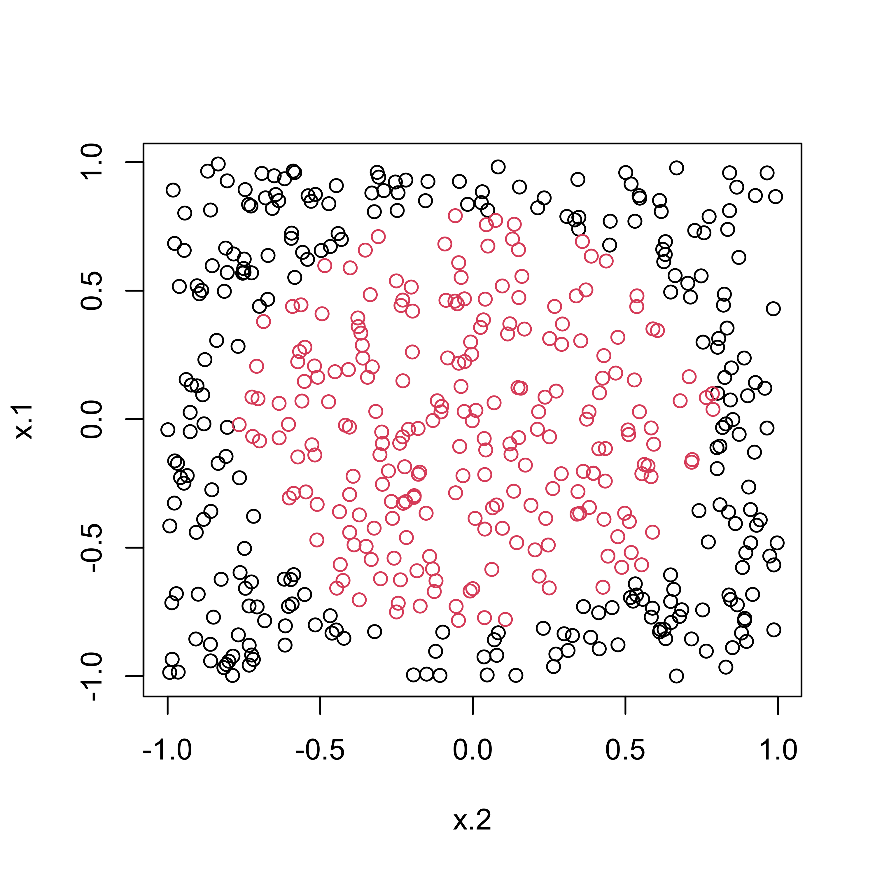
Circle Data Classification

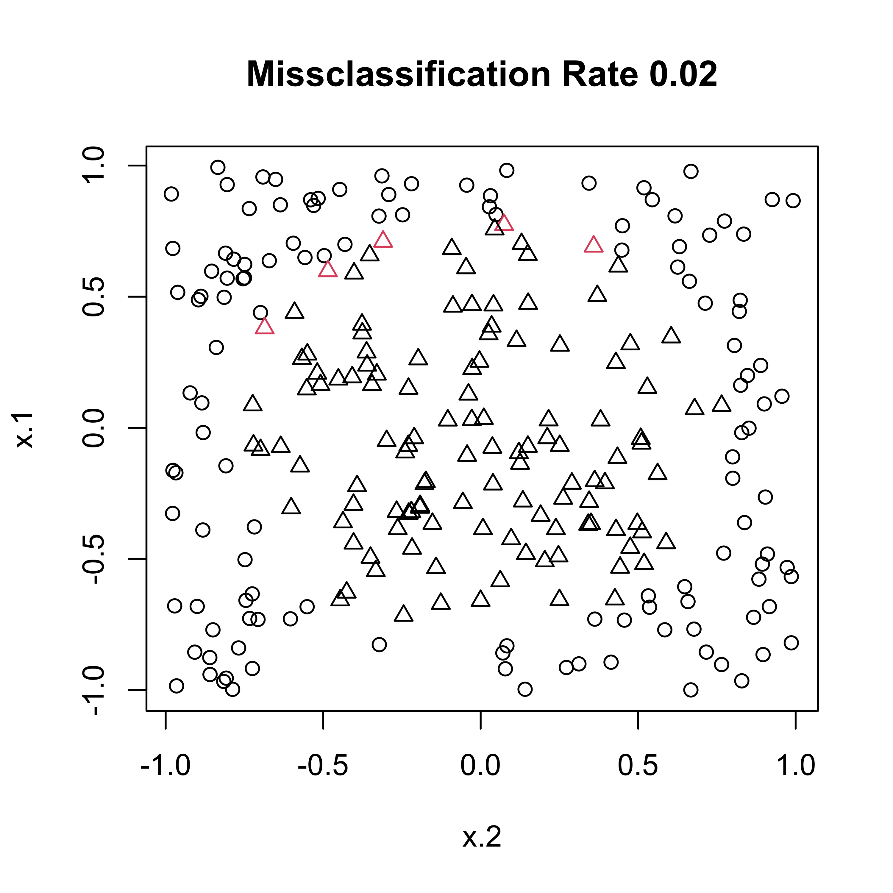
BARK Classification
classification = TRUEfor probit regressionselection = TRUEallows some of the \(\lambda_j\) to be 0common_lambdas = TRUEsets all (non-zero) \(\lambda_j\) to a common \(\lambda\)
Missclassification

Support Vector Machines (SVM) & BART
library(e1071)
circle2.svm = svm(y ~ x.1 + x.2, data=circle2[train,],
                  type="C")
pred.svm = predict(circle2.svm, circle2[-train,])
mean(pred.svm != circle2[-train, "y"])
[1] 0.048[1] 0.036Comparisons
| Data Sets | n | p | BARK-D | BARK-SE | BARK-SD | SVM | BART |
|---|---|---|---|---|---|---|---|
| Circle 2 | 200 | 2 | 4.91% | 1.88% | 1.93% | 5.03% | 3.97% |
| Circle 5 | 200 | 5 | 4.70% | 1.47% | 1.65% | 10.99% | 6.51% |
| Circle 20 | 200 | 20 | 4.84% | 2.09% | 3.69% | 44.10% | 15.10% |
| Bank | 200 | 6 | 1.25% | 0.55% | 0.88% | 1.12% | 0.50% |
| BC | 569 | 30 | 4.02% | 2.49% | 6.09% | 2.70% | 3.36% |
| Ionosphere | 351 | 33 | 8.59% | 5.78% | 10.87% | 5.17% | 7.34% |
- BARK-D: different \(\lambda_d\) for each dimension
- BARK-SE: selection and equal \(\lambda_d\) for non-zero \(\lambda_d\)
- BARK-SD: selection and different \(\lambda_d\) for non-zero \(\lambda_d\)
Needs & Limitations
- NP Bayes of many flavors often does better than frequentist methods (BARK, BART, Treed GP, more)
- Hyper-parameter specification - theory & computational approximation
- asymptotic theory (rates of convergence)
- need faster code for BARK that is easier for users (BART & TGP are great!)
- Can these models be added to JAGS, STAN, etc instead of stand-alone R packages
- With availability of code what are caveats for users?
Summary
Lévy Random Field Priors & LARK/BARK models:
- Provide limit of finite dimensional priors (GRP & SVSS) to infinite dimensional setting
- Adaptive bandwidth for kernel regression
- Allow flexible generating functions
- Provide sparser representations compared to SVM & RVM, with coherent Bayesian interpretation
- Incorporation of prior knowledge if available
- Relax assumptions of equally spaced data and Gaussian likelihood
- Hierarchical Extensions
- Formulation allows one to define stochastic processes on arbitrary spaces (spheres, manifolds)