Lecture 22: Nonparametric Regression

STA702

Merlise Clyde

Duke University

Semi-parametric Regression

Consider model \[Y_1, \dots, Y_n \sim \textsf{N}\left(\mu(\mathbf{x}_i, \boldsymbol{\theta}), \sigma \right)\]
Mean function \(\textsf{E}[Y_i \mid \boldsymbol{\theta}] = \mu(\mathbf{x}_i, \boldsymbol{\theta})\) falls in some class of nonlinear functions
Basis Function Expansion \[\mu(\mathbf{x}, \boldsymbol{\theta}) = \sum_{j = 1}^{J} \beta_j b_j(\mathbf{x})\]
\(b_j(\mathbf{x})\) is a pre-specified set of basis functions and \(\boldsymbol{\beta}= (\beta_1, \ldots, \beta_J)^T\) is a vector of coefficients or coordinates wrt to the basis

Examples

Taylor Series expansion of \(\mu(\mathbf{x})\) about point \(\chi\) \[\begin{aligned} \mu(x) & = \sum_k \frac{\mu^{(k)}(\chi)}{k!} (x - \chi)^k \\ & = \sum_k \beta_k (x - \chi)^k \end{aligned} \]
polynomial basis
can require a large number of terms to model globally
can have really poor behavior in regions without data
each basis function has a “global” impact

Other Basis Functions

cubic splines \[ b_j(x, \chi_j) = (x - \chi_j)^3_+\]
Gaussian Radial Basis \[ b_j(x, \chi_j) = \exp{\left(\frac{(x - \chi_j)^2}{l^2}\right)}\]
centers of basis functions \(\chi_j\)
width parameter \(l\) controls the scale at which the mean function dies out as a function of \(\mathbf{x}\) from the center
localized basis elements

Local Models

Multivariate Gaussian Kernel \(g\) with parameters \(\boldsymbol{\omega}= (\boldsymbol{\chi}, \boldsymbol{\Lambda})\) \[ b_j(\mathbf{x}, \boldsymbol{\omega}_j) = g( \boldsymbol{\Lambda}_j^{1/2} (\mathbf{x}- \boldsymbol{\chi}_j)) = \exp\left\{-\frac{1}{2}(\mathbf{x}- \boldsymbol{\chi}_j)^T \boldsymbol{\Lambda}_j (\mathbf{x}- \boldsymbol{\chi}_j)\right\} \]
Gaussian, Cauchy, Exponential, Double Exponential kernels (can be asymmetric)
translation and scaling of wavelet families
basis functions formed from a generator function \(g\) with location and scaling parameters

Bayesian Nonparametric Model

Mean function \[\mu(\mathbf{x}_i) = \sum_{j}^J b_j(\mathbf{x}_i, \boldsymbol{\omega}_j) \beta_j\]

conditional on the basis elements back to our Bayesian regression model
usually uncertainty about number of basis elements needed
could use BMA or other shrinkage priors
how should coefficients scale as \(J\) increases?
choice of \(J\)?
what about uncertainty in \(\boldsymbol{\omega}\) (locations and scales)?
priors on unknowns (\(J\), \(\{\beta_j\}\), \(\{\boldsymbol{\omega}_j\}\)) induces a prior on functions!

Stochastic Expansions

\[\mu(\mathbf{x}) = \sum_{j=0}^{J} b_j(\mathbf{x}, \boldsymbol{\omega}_j) \beta_j = \sum_{j=0}^{J} g(\boldsymbol{\Lambda}^{1/2}(\mathbf{x}- \boldsymbol{\omega}_j)) \beta_j \]

introduce a Lévy measure \(\nu( d\beta, d \boldsymbol{\omega})\)
Poisson distribution \(J \sim \textsf{Poi}(\nu_+)\) where \(\nu_+\equiv \nu(\mathbb{R}\times\boldsymbol{\Omega}) = \iint \nu(\beta, \boldsymbol{\omega}) d \beta \, d\boldsymbol{\omega}\)
conditional prior on \(\beta_j,\boldsymbol{\omega}_j \mid J \mathrel{\mathop{\sim}\limits^{\rm iid}}\pi(\beta, \boldsymbol{\omega}) \propto \nu(\beta,\boldsymbol{\omega})\)
Conditions on \(\nu\) (and \(g\))
- need to have that \(|\beta_j|\) are absolutely summable
- finite number of large coefficients (in absolute value)
- allows an infinite number of small \(\beta_j \in [-\epsilon, \epsilon]\)

See Wolpert, Clyde and Tu (2011) AoS

Gamma Process Example

\(\nu(\beta, \chi) = \beta^{-1} e^{- \beta \eta} \gamma(\chi) d \beta \, d \chi\) 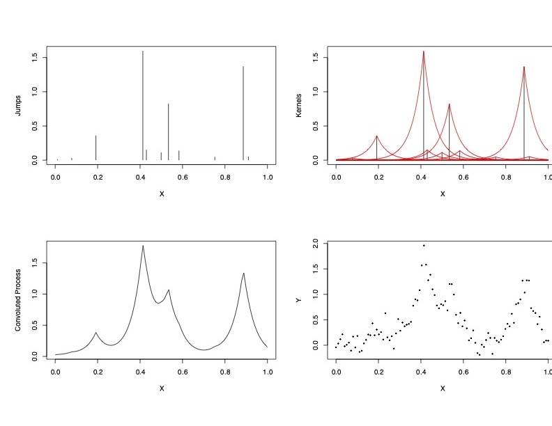convolution of a gamma process

Stochastic Integral Representation

\[\mu(\mathbf{x}) = \sum_{j=0}^{J} b_j(\mathbf{x}, \boldsymbol{\omega}_j) \beta_j = \sum_{j=0}^{J} g(\boldsymbol{\Lambda}^{1/2}(\mathbf{x}- \boldsymbol{\omega}_j)) \beta_j = \int_{\boldsymbol{\Omega}} b(\mathbf{x}, \boldsymbol{\omega}) {\cal L}(d\boldsymbol{\omega})\]

\({\cal L}\) is a random signed measure (generalization of Completely Random Measures) \[ {\cal L}\sim \textsf{Lévy}(\nu) \qquad \qquad {\cal L}(d \boldsymbol{\omega}) = \sum_{j \le J}\beta_j \delta_{\boldsymbol{\omega}_j} (d \boldsymbol{\omega})\]
Lévy-Khinchine Poisson Representation of \({\cal L}\)
Poisson number of support points (possibly infinite!)
random support points of discrete measure \(\{ \boldsymbol{\omega}_j\}\)
random “jumps” \(\beta_j\)
Convenient to think of a random measure as stochastic process where \({\cal L}\) assigns random variables to sets \(A \in \boldsymbol{\Omega}\)

Examples

gamma process \[\begin{aligned} \nu(\beta, \boldsymbol{\omega}) & = \beta^{-1} e^{- \beta \eta} \pi(\boldsymbol{\omega}) d \beta \, d \boldsymbol{\omega}\\ {\cal L}(A) & \sim \textsf{Gamma}(\pi(A), \eta) \end{aligned}\]
non-negative coefficients plus non-negative basis functions allows priors on non-negative functions without transformations
\(\alpha\)-Stable process (Cauchy process is \(\alpha = 1\)) \[\nu(\beta, \boldsymbol{\omega}) = c_\alpha |\beta|^{-(\alpha +1)}\ \pi(\boldsymbol{\omega}) \qquad 0 < \alpha < 2 \]
\(\nu^+(\mathbb{R}, \boldsymbol{\Omega}) = \infty\) for both the Gamma and \(\alpha\)-Stable processes
Fine in theory, but problematic for MCMC!

Prior Approximation I

Truncate measure \(\nu\) to obtain a finite expansion:

Finite number of support points \(\boldsymbol{\omega}\) with \(\beta\) in \([-\epsilon, \epsilon]^c\)
Fix \(\epsilon\) (for given prior approximation error)
Use approximate Lévy measure \(\nu_{\epsilon}(\beta, \boldsymbol{\omega}) \equiv \nu(\beta, \boldsymbol{\omega})\mathbf{1}(|\beta| > \epsilon)\)
\(\Rightarrow\) \(J \sim \textsf{Poi}(\nu_{\epsilon}^+)\) where \(\nu^+_{\epsilon} = \nu([-\epsilon, \epsilon]^c, \boldsymbol{\Omega})\)
\(\Rightarrow\) \(\beta_j, \boldsymbol{\omega}_j \mathrel{\mathop{\sim}\limits^{\rm iid}}\pi(d\beta, d\boldsymbol{\omega}) \equiv \nu_\epsilon(d\beta , d \boldsymbol{\omega})/\nu^+_{\epsilon}\)
for \(\alpha\)-Stable, the approximation leads to double Pareto distributions for \(\beta\) \[\pi(\beta_j) = \frac{\epsilon}{2 \eta} |\beta|^{- \alpha - 1} \mathbf{1}_{|\beta| > \frac{\boldsymbol{\epsilon}}{\eta}}\]

Truncated Cauchy Process Prior

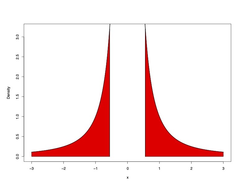
Truncated Cauchy

Simulation

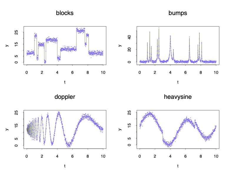
Kernels

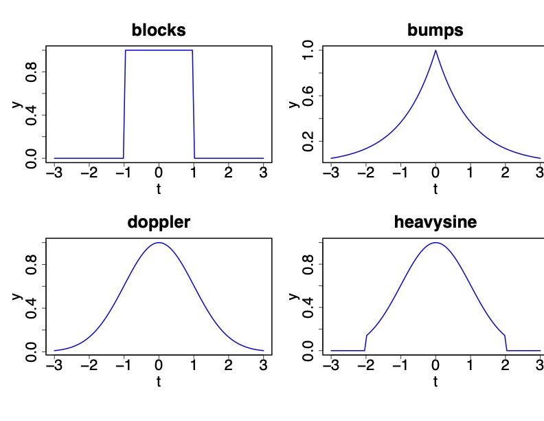
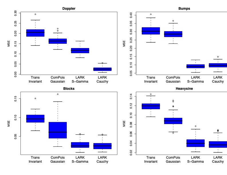
Comparison of Lévy Adaptive Regression Kernels

Inference via Reversible Jump MCMC

trans-dimensional MCMC

number of support points \(J\) varies from iteration to iteration
- add a new point (birth)
- delete an existing point (death)
- combine two points (merge)
- split a point into two
update existing point(s)

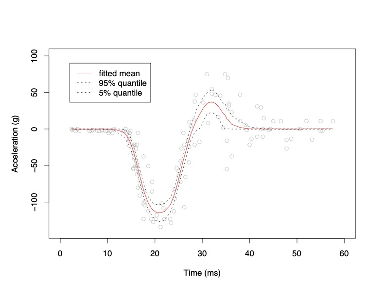
MotorCycle Acceleration

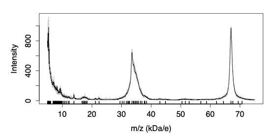
Mass Spectroscopy

Summary

more parsimonious than “shrinkage” priors or SVM
allows for increasing number of support points as \(n\) increases
control MSE a priori through choice of \(\epsilon\)
no problem with non-normal data, non-negative functions or even discontinuous functions
credible and prediction intervals
robust alternative to Gaussian Process Priors
hard to scale up random scales, locations as dimension of \(\mathbf{x}\) increases
next - Prior Approximation II