Lecture 16: Bayesian Variable Selection and Model Averaging

STA702

Merlise Clyde

Duke University

Normal Regression Model

Centered regression model where \(\mathbf{X}^c\) is the \(n \times p\) centered design matrix where all variables have had their means subtracted (may or may not need to be standardized)

\[\mathbf{Y}= \mathbf{1}_n \alpha + \mathbf{X}^c \boldsymbol{\beta}+ \boldsymbol{\epsilon}\]

• “Redundant” variables lead to unstable estimates
  

• Some variables may not be relevant at all (\(\beta_j = 0\))

• We want to reduce the dimension of the predictor space

• How can we infer a “good” model that uses a subset of predictors from the data?

• Expand model hierarchically to introduce another latent variable \(\boldsymbol{\gamma}\) that encodes models \({\cal M}_\gamma\) \(\boldsymbol{\gamma}= (\gamma_1, \gamma_2, \ldots \gamma_p)^T\) where \[\begin{align*} \gamma_j = 0 & \Leftrightarrow \beta_j = 0 \\ \gamma_j = 1 & \Leftrightarrow \beta_j \neq 0 \end{align*}\]

• Find Bayes factors and posterior probabilities of models \({\cal M}_\gamma\)

Priors

With \(2^p\) models, subjective priors for \(\boldsymbol{\beta}\) are out of the question for moderate \(p\) and improper priors lead to arbitrary Bayes factors leading to conventional priors on model specific parameters

• Zellner’s g-prior and related have attractive properties as a starting point \[\boldsymbol{\beta}_\gamma \mid \alpha, \phi, \boldsymbol{\gamma}\sim \textsf{N}(0, g \phi^{-1} ({\mathbf{X}_{\boldsymbol{\gamma}}^c}^\prime \mathbf{X}_{\boldsymbol{\gamma}}^c)^{-1})\]

• Independent Jeffrey’s prior on common parameters \((\alpha, \phi)\)
  \(p(\alpha, \phi) \propto 1/\phi\)

• marginal likelihood of \(\boldsymbol{\gamma}\) that is proportional to \[ p(\mathbf{Y}\mid \boldsymbol{\gamma}) = C (1 + g)^{\frac{n-p_{\boldsymbol{\gamma}}-1}{2}} ( 1 + g (1 - R^2_\gamma))^{- \frac{(n-1)}{2}}\]

• \(R^2_\gamma\) is the usual coefficient of determination for model \({\cal M}_\gamma\).

• \(C\) is a constant common to all models (proportional to the marginal likelihood of the null model where \(\boldsymbol{\beta_\gamma}= \mathbf{0}_p\)

Sketch for Marginal

• Integrate out \(\boldsymbol{\beta_\gamma}\) using sums of normals
  
• Find inverse of \(\mathbf{I}_n + g \mathbf{P}_{\mathbf{X}_{\boldsymbol{\gamma}}}\) (properties of projections or Sherman-Woodbury-Morrison Theorem)
  
• Find determinant of \(\phi (\mathbf{I}_n + g \mathbf{P}_{\mathbf{X}_{\boldsymbol{\gamma}}})\)
  
• Integrate out intercept (normal)
  
• Integrate out \(\phi\) (gamma)
  
• algebra to simplify quadratic forms to \(R^2_{\boldsymbol{\gamma}}\)

Or integrate \(\alpha\), \(\boldsymbol{\beta_\gamma}\) and \(\phi\) (complete the square!)

Posterior Distributions on Parameters

\[\begin{align*}\alpha \mid \boldsymbol{\gamma}, \phi, y & \sim \textsf{N}\left(\bar{y}, \frac{1}{n \phi}\right)\\ \boldsymbol{\beta}_{\boldsymbol{\gamma}} \mid \boldsymbol{\gamma}, \phi, g, y &\sim \textsf{N}\left( \frac{g}{1 + g} \hat{\boldsymbol{\beta}}_{\gamma}, \frac{g}{1 + g} \frac{1}{\phi} \left[{\boldsymbol{X}_{\gamma}}^T \boldsymbol{X}_{\gamma} \right]^{-1} \right) \\ \phi \mid \gamma, y & \sim \textsf{Gamma}\left(\frac{n-1}{2}, \frac{\textsf{TotalSS} - \frac{g}{1+g} \textsf{RegSS}}{2}\right) \\ \textsf{TotalSS} & \equiv \sum_i (y_i - \bar{y})^2 \\ \textsf{RegSS} & \equiv \hat{\boldsymbol{\beta}}_\gamma^T \boldsymbol{X}_\gamma^T \boldsymbol{X}_\gamma \hat{\beta}\gamma \\ R^2_\gamma & = \frac{\textsf{RegSS}}{\textsf{TotalSS}} = 1 - \frac{\textsf{ErrorSS}}{\textsf{TotalSS}} \end{align*}\]

Priors on Model Space

\(p({\cal M}_\gamma) \Leftrightarrow p(\boldsymbol{\gamma})\)

• Fixed prior probability \(\gamma_j\) \(p(\gamma_j = 1) = .5 \Rightarrow P({\cal M}_\gamma) = .5^p\)

• Uniform on space of models \(p_{\boldsymbol{\gamma}}\sim \textsf{Bin}(p, .5)\)

• Hierarchical prior \[\begin{align} \gamma_j \mid \pi & \mathrel{\mathop{\sim}\limits^{\rm iid}}\textsf{Ber}(\pi) \\ \pi & \sim \textsf{Beta}(a,b) \\ \text{then } p_{\boldsymbol{\gamma}}& \sim \textsf{BB}_p(a, b) \end{align}\]

\[ p(p_{\boldsymbol{\gamma}}\mid p, a, b) = \frac{ \Gamma(p + 1) \Gamma(p_{\boldsymbol{\gamma}}+ a) \Gamma(p - p_{\boldsymbol{\gamma}}+ b) \Gamma (a + b) }{\Gamma(p_{\boldsymbol{\gamma}}+1) \Gamma(p - p_{\boldsymbol{\gamma}}+ 1) \Gamma(p + a + b) \Gamma(a) \Gamma(b)} \] - Uniform on Model Size \(\Rightarrow p_{\boldsymbol{\gamma}}\sim \textsf{BB}_p(1, 1) \sim \textsf{Unif}(0, p)\)

Posterior Probabilities of Models

• Calculate posterior distribution analytically under enumeration. \[p({\cal M}_\gamma\mid \mathbf{Y})= \frac{p(\mathbf{Y}\mid \boldsymbol{\gamma}) p(\boldsymbol{\gamma})} {\sum_{\boldsymbol{\gamma}^\prime \in \Gamma} p(\mathbf{Y}\mid \boldsymbol{\gamma}^\prime) p(\boldsymbol{\gamma}^\prime)}\]

• Express as a function of Bayes factors and prior odds!

• Use MCMC over \(\Gamma\) - Gibbs, Metropolis Hastings if \(p\) is large (depends on Bayes factors and prior odds)

• slow convergence/poor mixing with high correlations
  

• Metropolis Hastings algorithms more flexibility
  (swap pairs of variables)

No need to run MCMC over \(\boldsymbol{\gamma}\), \(\boldsymbol{\beta_\gamma}\), \(\alpha\), and \(\phi\)!

Choice of \(g\): Bartlett’s Paradox

The Bayes factor for comparing \(\boldsymbol{\gamma}\) to the null model: \[ BF(\boldsymbol{\gamma}: \boldsymbol{\gamma}_0) = (1 + g)^{(n - 1 - p_{\boldsymbol{\gamma}})/2} (1 + g(1 - R_{\boldsymbol{\gamma}}^2))^{-(n-1)/2} \]

• For fixed sample size \(n\) and \(R_{\boldsymbol{\gamma}}^2\), consider taking values of \(g\) that go to infinity
  
• Increasing vagueness in prior
• What happens to BF as \(g \to \infty\)?

Bartlett Paradox

Why is this a paradox?

Information Paradox

The Bayes factor for comparing \(\boldsymbol{\gamma}\) to the null model: \[ BF(\boldsymbol{\gamma}: \boldsymbol{\gamma}_0) = (1 + g)^{(n - 1 - p_{\boldsymbol{\gamma}})/2} (1 + g(1 - R_{\boldsymbol{\gamma}}^2))^{-(n-1)/2} \]

• Let \(g\) be a fixed constant and take \(n\) fixed.
  
• Usual F statistic for testing \(\boldsymbol{\gamma}\) versus \(\boldsymbol{\gamma}_0\) is \(F = \frac{R_{\boldsymbol{\gamma}}^2/p_{\boldsymbol{\gamma}}}{(1 - R_{\boldsymbol{\gamma}}^2)/(n - 1 - p_{\boldsymbol{\gamma}})}\)
  
• As \(R^2_{\boldsymbol{\gamma}} \to 1\), \(F \to \infty\) Likelihood Rqtio test (F-test) would reject \(\boldsymbol{\gamma}_0\) where \(F\) is the usual \(F\) statistic for comparing model \(\boldsymbol{\gamma}\) to \(\boldsymbol{\gamma}_0\)
  
• BF converges to a fixed constant \((1+g)^{n - 1 -p_{\boldsymbol{\gamma}}/2}\) (does not go to infinity !

Information Inconsistency of Liang et al JASA 2008

Mixtures of \(g\)-priors & Information consistency

• Want \(\textsf{BF}\to \infty\) if \(\textsf{R}_{\boldsymbol{\gamma}}^2 \to 1\) if model is full rank
• Put a prior on \(g\) \[BF(\boldsymbol{\gamma}: \boldsymbol{\gamma}_0) = \frac{ C \int (1 + g)^{(n - 1 - p_{\boldsymbol{\gamma}})/2} (1 + g(1 - R_{\boldsymbol{\gamma}}^2))^{-(n-1)/2} \pi(g) dg}{C}\]
• interchange limit and integration as \(R^2 \to 1\) want \[ \textsf{E}_g[(1 + g)^{(n-1-p_{\boldsymbol{\gamma}})/2}]\] to diverge under the prior

One Solution

• hyper-g prior (Liang et al JASA 2008) \[p(g) = \frac{a-2}{2}(1 + g)^{-a/2}\] or \(g/(1+g) \sim Beta(1, (a-2)/2)\) for \(a > 2\)

• prior expectation converges if \(a > n + 1 - p_{\boldsymbol{\gamma}}\) (properties of \(_2F_1\) function)

• Consider minimal model \(p_{\boldsymbol{\gamma}}= 1\) and \(n = 3\) (can estimate intercept, one coefficient, and \(\sigma^2\), then for \(a > 3\) integral exists

• For \(2 < a \le 3\) integral diverges and resolves the information paradox! (see proof in Liang et al JASA 2008 )

Examples of Priors on \(g\)

• hyper-g prior (Liang et al JASA 2008)

  • Special case is Jeffreys prior for \(g\) which corresponds to \(a = 2\) (improper)
    

• Zellner-Siow Cauchy prior \(1/g \sim \textsf{Gamma}(1/2, n/2)\)
  

• Hyper-g/n \((g/n)(1 + g/n) \sim \textsf{Beta}(1, (a-2)/2)\) (generalized Beta distribution)

• robust prior (Bayarri et al Annals of Statistics 2012 )

• Intrinsic prior (Womack et al JASA 2015)

All have prior tails for \(\boldsymbol{\beta}\) that behave like a Cauchy distribution and all except the Gamma prior have marginal likelihoods that can be computed using special hypergeometric functions (\(_2F_1\), Appell \(F_1\))

No fixed value of \(g\) (i.e a point mass prior) will resolve!

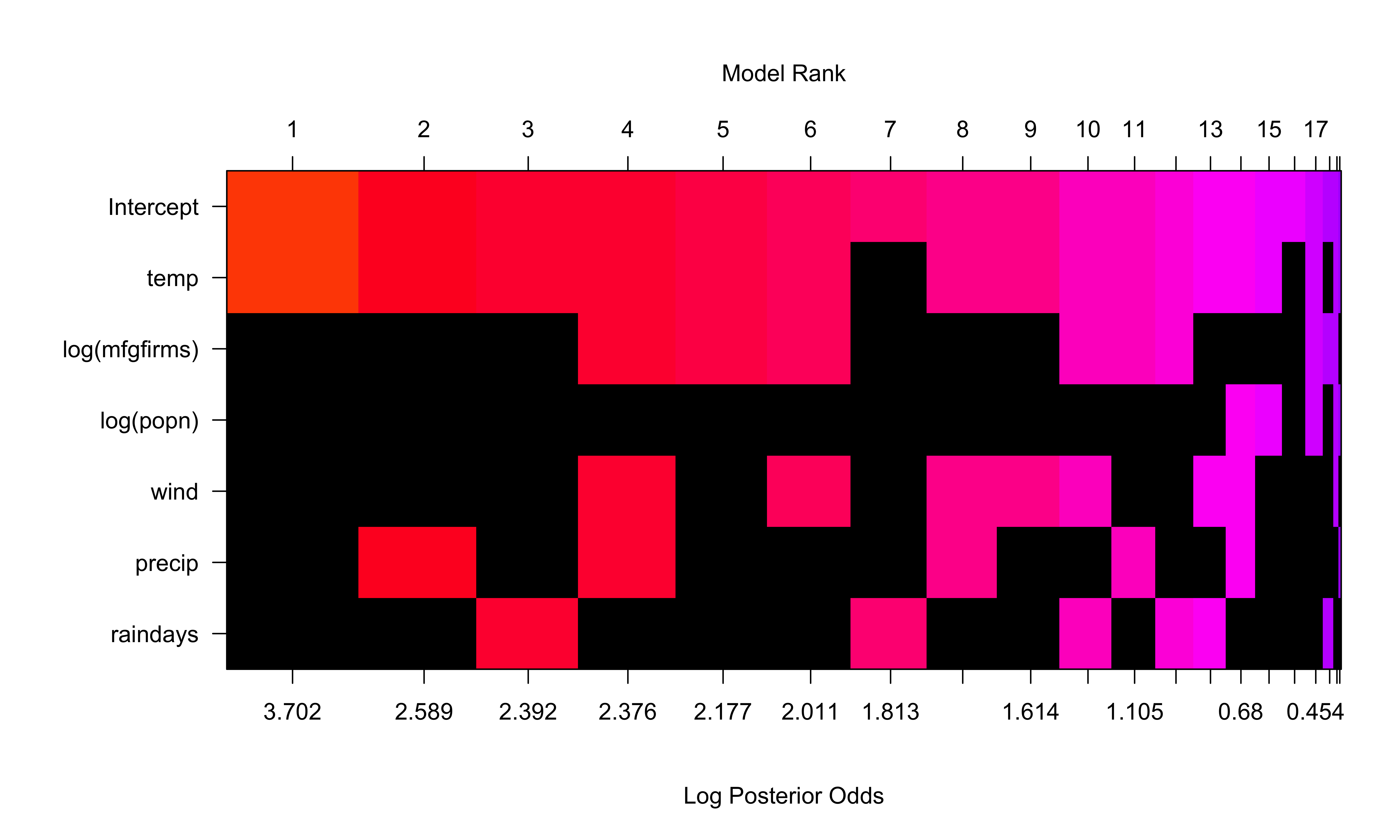
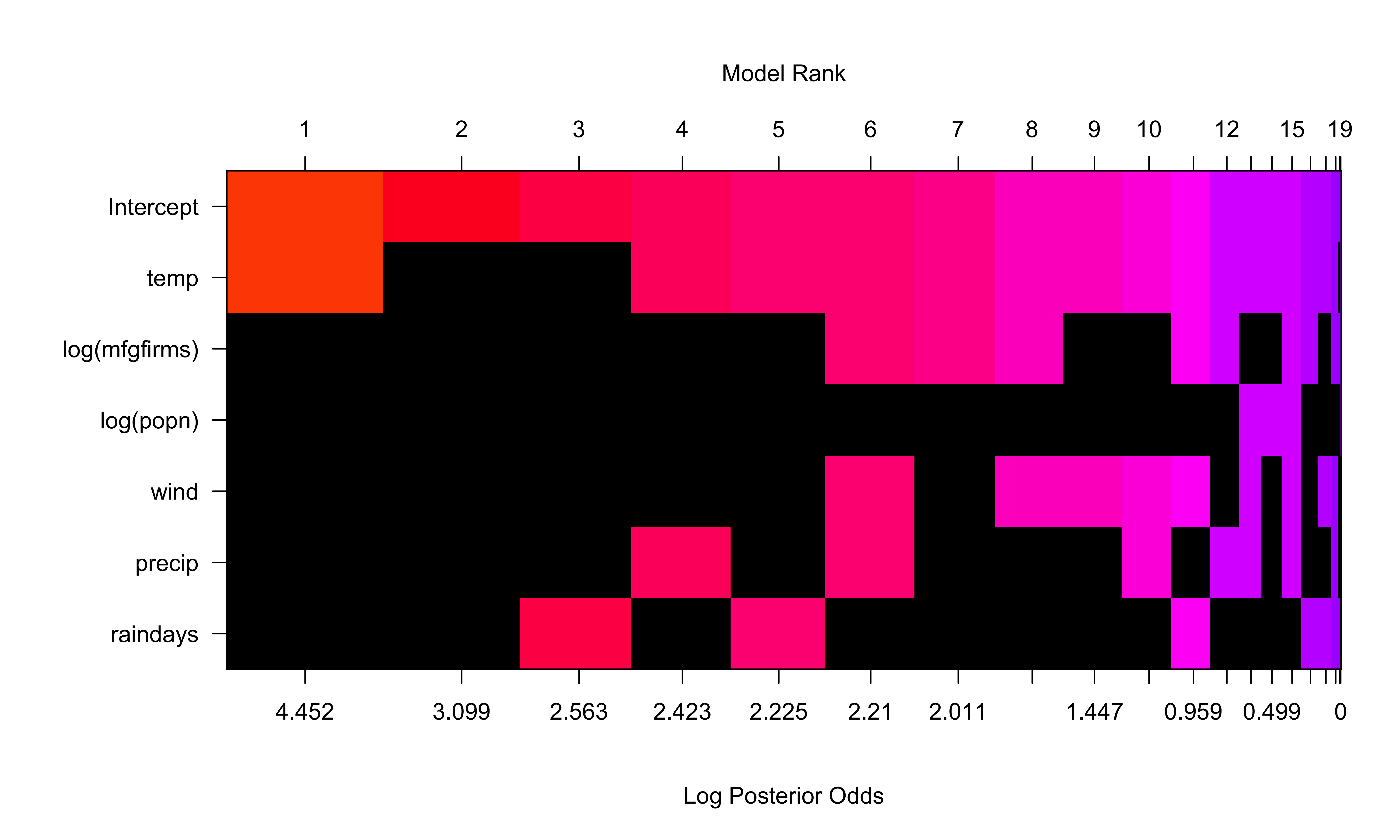
US Air Example

library(BAS)
data(usair, package="HH")
poll.bma = bas.lm(log(SO2) ~ temp + log(mfgfirms) +
                             log(popn) + wind +
                             precip + raindays,
                  data=usair,
                  prior="JZS",  #Jeffrey-Zellner-Siow
                  alpha=nrow(usair), # n
                  n.models=2^6,
                  modelprior = uniform(),
                  method="deterministic")

Summary

summary(poll.bma, n.models=4)

              P(B != 0 | Y) model 1   model 2   model 3   model 4
Intercept        1.00000000 1.00000 1.0000000 1.0000000 1.0000000
temp             0.91158530 1.00000 1.0000000 1.0000000 1.0000000
log(mfgfirms)    0.31718916 0.00000 0.0000000 0.0000000 1.0000000
log(popn)        0.09223957 0.00000 0.0000000 0.0000000 0.0000000
wind             0.29394451 0.00000 0.0000000 0.0000000 1.0000000
precip           0.28384942 0.00000 1.0000000 0.0000000 1.0000000
raindays         0.22903262 0.00000 0.0000000 1.0000000 0.0000000
BF                       NA 1.00000 0.3286643 0.2697945 0.2655873
PostProbs                NA 0.29410 0.0967000 0.0794000 0.0781000
R2                       NA 0.29860 0.3775000 0.3714000 0.5427000
dim                      NA 2.00000 3.0000000 3.0000000 5.0000000
logmarg                  NA 3.14406 2.0313422 1.8339656 1.8182487

Plots of Coefficients

 beta = coef(poll.bma)
 par(mfrow=c(2,3));  plot(beta, subset=2:7,ask=F)

Posterior Distribution with Uniform Prior on Model Space

image(poll.bma, rotate=FALSE)

Posterior Distribution with BB(1,1) Prior on Model Space

poll.bb.bma = bas.lm(log(SO2) ~ temp + log(mfgfirms) +
                                log(popn) + wind +
                                precip + raindays,
                     data=usair,
                     prior="JZS",
                     alpha=nrow(usair),
                     n.models=2^6,  #enumerate
                     modelprior=beta.binomial(1,1))

Posterior Distribution with BB(1,1) Prior on Model Space

image(poll.bb.bma, rotate=FALSE)

Summary

• Choice of prior on \(\boldsymbol{\beta_\gamma}\)
• g-priors or mixtures of \(g\) (sensitivity)
• priors on the models (sensitivity)
• posterior summaries - select a model or “average” over all models