Lecture 14: Basics of Bayesian Hypothesis Testing

STA702

Merlise Clyde

Duke University

Feature Selection via Shrinkage

• modal estimates in regression models under certain shrinkage priors will set a subset of coefficients to zero

• not true with posterior mean

• multi-modal posterior

• no prior probability that coefficient is zero

• how should we approach selection/hypothesis testing?

• Bayesian Hypothesis Testing

Basics of Bayesian Hypothesis Testing

Suppose we have univariate data \(Y_i \overset{iid}{\sim} \mathcal{N}(\theta, 1)\), \(\mathbf{Y}= (y_i, \ldots, y_n)^T\)

• goal is to test \(\mathcal{H}_0: \theta = 0; \ \ \text{vs } \mathcal{H}_1: \theta \neq 0\)

• Additional unknowns are \(\mathcal{H}_0\) and \(\mathcal{H}_1\)

• Put a prior on the actual hypotheses/models, that is, on \(\pi(\mathcal{H}_0) = \Pr(\mathcal{H}_0 = \text{True})\) and \(\pi(\mathcal{H}_1) = \Pr(\mathcal{H}_1 = \text{True})\).

• (Marginal) Likelihood of the hypotheses: \(\cal{L}(\mathcal{H}_i) \propto p( \mathbf{y}\mid \mathcal{H}_i)\)

\[p( \mathbf{y}\mid \mathcal{H}_0) = \prod_{i = 1}^n (2 \pi)^{-1/2} \exp{- \frac{1}{2} (y_i - 0)^2}\]

\[p( \mathbf{y}\mid \mathcal{H}_1) = \int_\Theta p( \mathbf{y}\mid \mathcal{H}_1, \theta) p(\theta \mid \mathcal{H}_1) \, d\theta\]

Bayesian Approach

• Need priors distributions on parameters under each hypothesis

  • in our simple normal model, the only additional unknown parameter is \(\theta\)
  • under \(\mathcal{H}_0\), \(\theta = 0\) with probability 1
  • under \(\mathcal{H}_0\), \(\theta \in \mathbb{R}\) we could take \(\pi(\theta) = \mathcal{N}(\theta_0, 1/\tau_0^2)\).

• Compute marginal likelihoods for each hypothesis, that is, \(\cal{L}(\mathcal{H}_0)\) and \(\cal{L}(\mathcal{H}_1)\).

• Obtain posterior probabilities of \(\cal{H}_0\) and \(\cal{H}_1\) via Bayes Theorem. \[ \begin{split} \pi(\mathcal{H}_1 \mid \mathbf{y}) = \frac{ p( \mathbf{y}\mid \mathcal{H}_1) \pi(\mathcal{H}_1) }{ p( \mathbf{y}\mid \mathcal{H}_0) \pi(\mathcal{H}_0) + p( \mathbf{y}\mid \mathcal{H}_1) \pi(\mathcal{H}_1)} \end{split} \]

• Provides a joint posterior distribution for \(\theta\) and \(\mathcal{H}_i\): \(p(\theta \mid \mathcal{H}_i, \mathbf{y})\) and \(\pi(\mathcal{H}_i \mid \mathbf{y})\)

Hypothesis Tests via Decision Theory

• Loss function for hypothesis testing

  • \(\hat{\cal{H}}\) is the chosen hypothesis

  • \(\cal{H}_{\text{true}}\) is the true hypothesis, \(\cal{H}\) for short

• Two types of errors:

  • Type I error: \(\hat{\cal{H}} = 1\) and \(\cal{H} = 0\)

  • Type II error: \(\hat{\cal{H}} = 0\) and \(\cal{H} = 1\)

• Loss function: \[L(\hat{\cal{H}}, \cal{H}) = w_1 \, 1(\hat{\cal{H}} = 1, \cal{H} = 0) + w_2 \, 1(\hat{\cal{H}} = 0, \cal{H} = 1)\]

  • \(w_1\) weights how bad it is to make a Type I error

  • \(w_2\) weights how bad it is to make a Type II error

Loss Function Functions and Decisions

• Relative weights \(w = w_2/w_1\) \[L(\hat{\cal{H}}, \cal{H}) = \, 1(\hat{\cal{H}} = 1, \cal{H} = 0) + w \, 1(\hat{\cal{H}} = 0, \cal{H} = 1)\]

• Special case \(w=1\) \[L(\hat{\cal{H}}, \cal{H}) = 1(\hat{\cal{H}} \neq \cal{H})\]

• known as 0-1 loss (most common)

• Bayes Risk (Posterior Expected Loss) \[\textsf{E}_{\cal{H} \mid \mathbf{y}}[L(\hat{\cal{H}}, \cal{H}) ] = 1(\hat{\cal{H}} = 1)\pi(\cal{H}_0 \mid \mathbf{y}) + 1(\hat{\cal{H}} = 0) \pi(\cal{H}_1 \mid \mathbf{y})\]

• Minimize loss by picking hypothesis with the highest posterior probability

Bayesian hypothesis testing

• Using Bayes theorem, \[ \begin{split} \pi(\mathcal{H}_1 \mid \mathbf{y}) = \frac{ p( \mathbf{y}\mid \mathcal{H}_1) \pi(\mathcal{H}_1) }{ p( \mathbf{y}\mid \mathcal{H}_0) \pi(\mathcal{H}_0) + p( \mathbf{y}\mid \mathcal{H}_1) \pi(\mathcal{H}_1)}, \end{split} \]

• If \(\pi(\mathcal{H}_0) = 0.5\) and \(\pi(\mathcal{H}_1) = 0.5\) a priori, then \[ \begin{split} \pi(\mathcal{H}_1 \mid \mathbf{y}) & = \frac{ 0.5 p( \mathbf{y}\mid \mathcal{H}_1) }{ 0.5 p( \mathbf{y}\mid \mathcal{H}_0) + 0.5 p( \mathbf{y}\mid \mathcal{H}_1) } \\ \\ & = \frac{ p( \mathbf{y}\mid \mathcal{H}_1) }{ p( \mathbf{y}\mid \mathcal{H}_0) + p( \mathbf{y}\mid \mathcal{H}_1) }= \frac{ 1 }{ \frac{p( \mathbf{y}\mid \mathcal{H}_0)}{p( \mathbf{y}\mid \mathcal{H}_1)} + 1 }\\ \end{split} \]

Bayes factors

• The ratio \(\frac{p( \mathbf{y}\mid \mathcal{H}_0)}{p( \mathbf{y}\mid \mathcal{H}_1)}\) is a ratio of marginal likelihoods and is known as the Bayes factor in favor of \(\mathcal{H}_0\), written as \(\mathcal{BF}_{01}\). Similarly, we can compute \(\mathcal{BF}_{10}\) via the inverse ratio.

• Bayes factors provide a weight of evidence in the data in favor of one model over another. and are used as an alternative to the frequentist p-value.

• Rule of Thumb: \(\mathcal{BF}_{01} > 10\) is strong evidence for \(\mathcal{H}_0\); \(\mathcal{BF}_{01} > 100\) is decisive evidence for \(\mathcal{H}_0\).

• In the example (with equal prior probabilities), \[ \begin{split} \pi(\mathcal{H}_1 \mid \mathbf{y}) = \frac{ 1 }{ \frac{p( \mathbf{y}\mid \mathcal{H}_0)}{p( \mathbf{y}\mid \mathcal{H}_1)} + 1 } = \frac{ 1 }{ \mathcal{BF}_{01} + 1 } \\ \end{split} \]

• the higher the value of \(\mathcal{BF}_{01}\), that is, the weight of evidence in the data in favor of \(\mathcal{H}_0\), the lower the marginal posterior probability that \(\mathcal{H}_1\) is true.

• \(\mathcal{BF}_{01} \uparrow\), \(\pi(\mathcal{H}_1 \mid \mathbf{y}) \downarrow\).

Posterior Odds and Bayes Factors

• Posterior odds \(\frac{\pi(\mathcal{H}_0 \mid \mathbf{y})}{\pi(\mathcal{H}_1 \mid \mathbf{y})}\) \[ \begin{split} \frac{\pi(\mathcal{H}_0 | \mathbf{y})}{\pi(\mathcal{H}_1 | \mathbf{y})} & = \frac{ p( \mathbf{y}|\mathcal{H}_0) \pi(\mathcal{H}_0) }{ p( \mathbf{y}| \mathcal{H}_0) \pi(\mathcal{H}_0) + p( \mathbf{y}| \mathcal{H}_1) \pi(\mathcal{H}_1)} \div \frac{ p( \mathbf{y}| \mathcal{H}_1) \pi(\mathcal{H}_1) }{ p( \mathbf{y}\mathcal{H}_0) \pi(\mathcal{H}_0) + p( \mathbf{y}| \mathcal{H}_1) \pi(\mathcal{H}_1)}\\ \\ & = \frac{ p( \mathbf{y}| \mathcal{H}_0) \pi(\mathcal{H}_0) }{ p( \mathbf{y}| \mathcal{H}_0) \pi(\mathcal{H}_0) + p( \mathbf{y}| \mathcal{H}_1) \pi(\mathcal{H}_1)} \times \frac{ p( \mathbf{y}| \mathcal{H}_0) \pi(\mathcal{H}_0) + p( \mathbf{y}| \mathcal{H}_1) \pi(\mathcal{H}_1)}{ p( \mathbf{y}| \mathcal{H}_1) \pi(\mathcal{H}_1) }\\ \\ \therefore \underbrace{\frac{\pi(\mathcal{H}_0 \mid \mathbf{y})}{\pi(\mathcal{H}_1 \mid \mathbf{y})}}_{\text{posterior odds}} & = \underbrace{\frac{ \pi(\mathcal{H}_0) }{ \pi(\mathcal{H}_1) }}_{\text{prior odds}} \times \underbrace{\frac{ p( \mathbf{y}\mid \mathcal{H}_0) }{ p( \mathbf{y}\mid \mathcal{H}_1) }}_{\text{Bayes factor } \mathcal{BF}_{01}} \\ \end{split} \]

• The Bayes factor can be thought of as the factor by which our prior odds change (towards the posterior odds) in the light of the data.

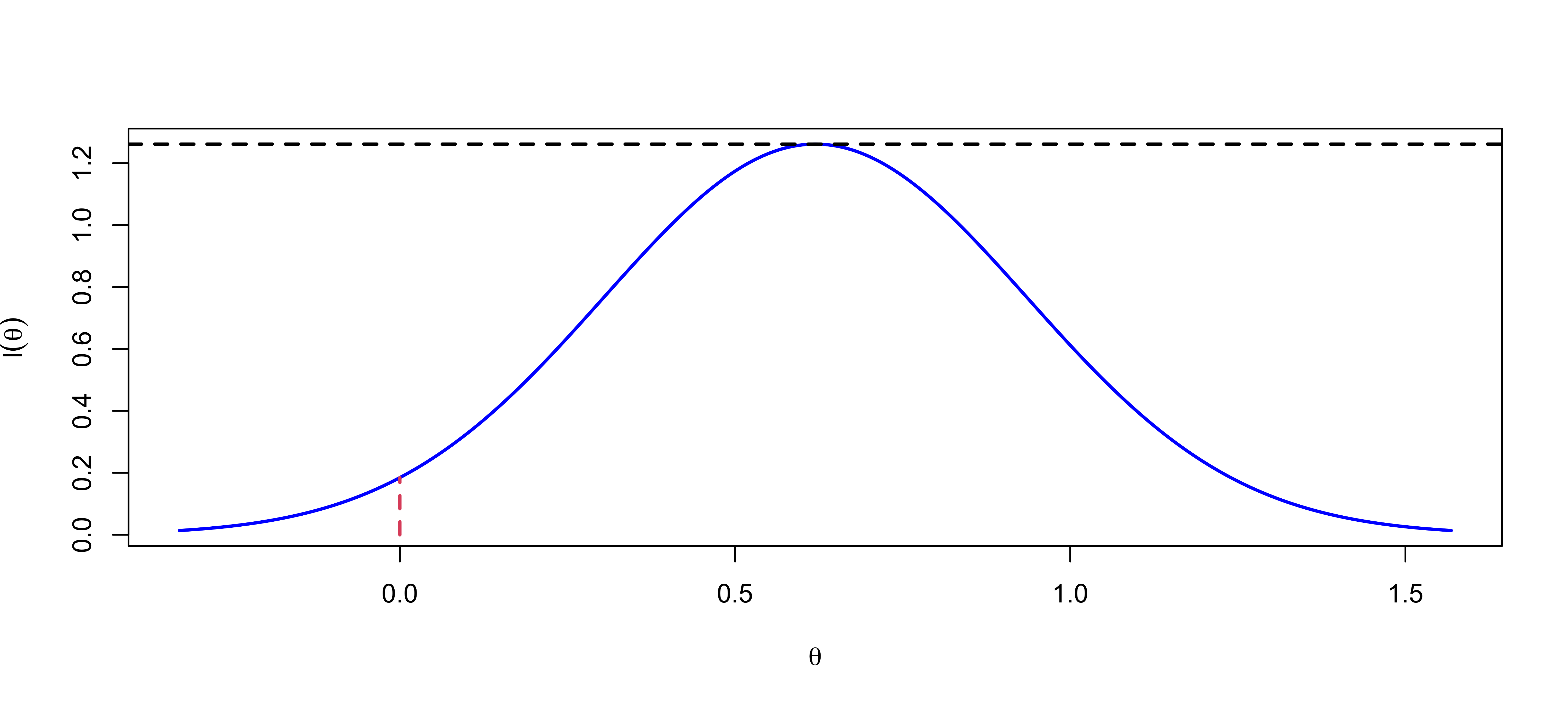
Likelihoods & Evidence

Maximized Likelihood. \(n = 10\)

p-value = 0.05

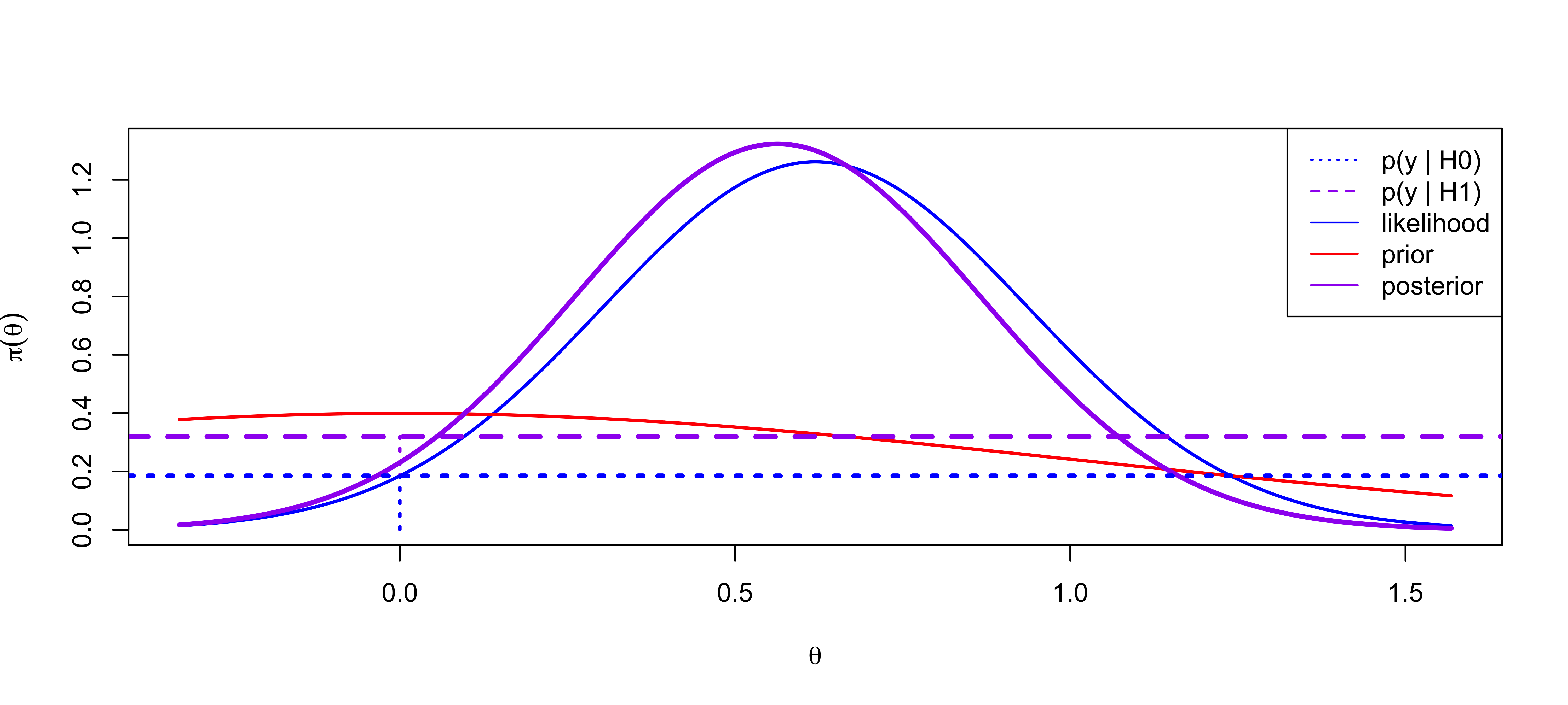
Marginal Likelihoods & Evidence

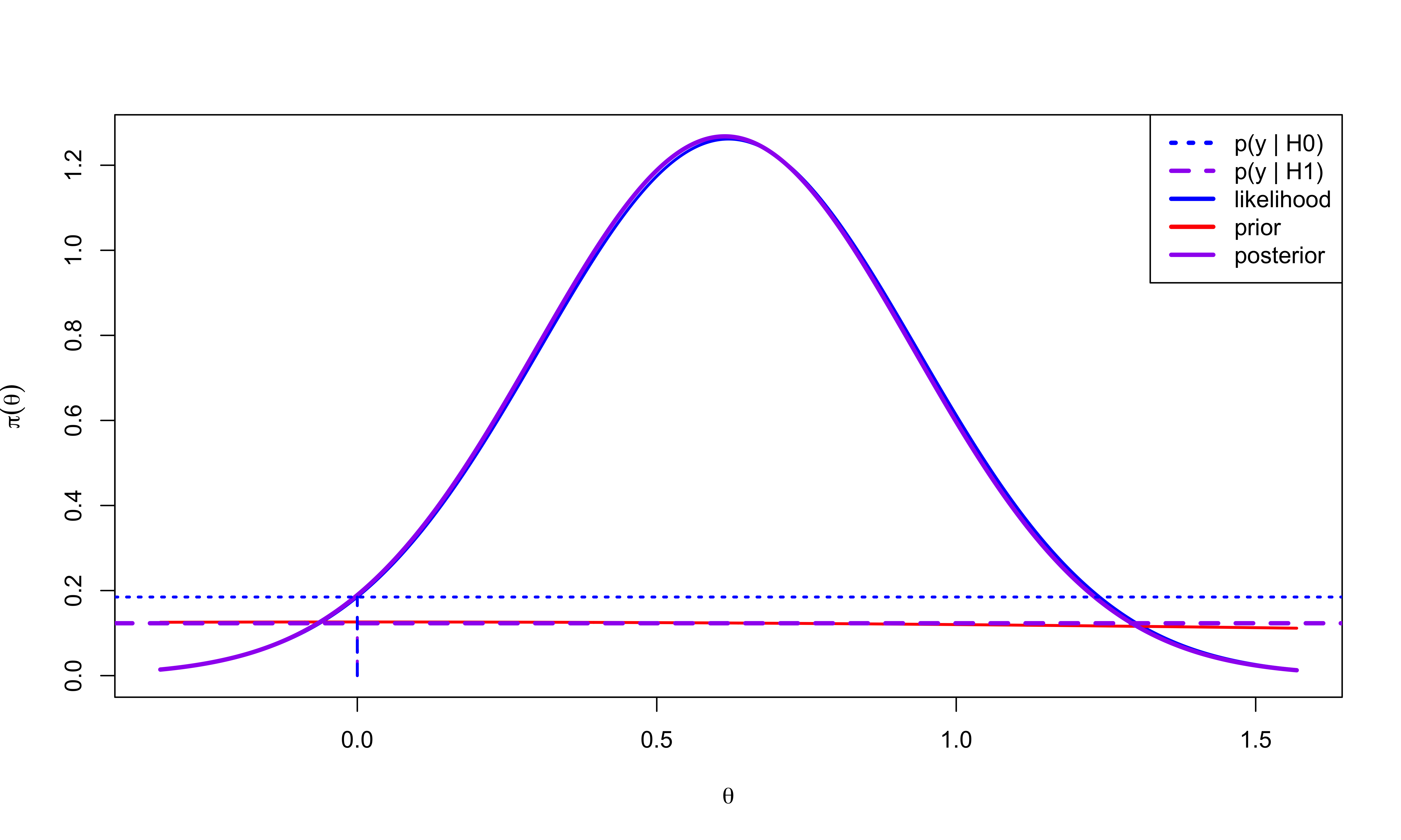
Maximized & Marginal Likelihoods

\(\cal{BF}_{10}\) = 1.73 or \(\cal{BF}_{01}\) = 0.58

Posterior Probability of \(\cal{H}_0\) = 0.3665

Candidate’s Formula (Besag 1989)

Alternative expression for BF based on Candidate’s Formula or Savage-Dickey ratio \[\cal{BF}_{01} = \frac{p( \mathbf{y}\mid \cal{H}_0)} {p( \mathbf{y}\mid \cal{H}_1)} = \frac{\pi_\theta(0 \mid \cal{H}_1, \mathbf{y})} {\pi_\theta(0 \mid \cal{H}_1)}\]

\[\pi_\theta(\theta \mid \cal{H}_i, \mathbf{y}) = \frac{p(\mathbf{y}\mid \theta, \cal{H}_i) \pi(\theta \mid \cal{H}_i)} {p(\mathbf{y}\mid \cal{H}_i)} \Rightarrow p(\mathbf{y}\mid \cal{H}_i) = \frac{p(\mathbf{y}\mid \theta, \cal{H}_i) \pi(\theta \mid \cal{H}_i)} {\pi_\theta(\theta \mid \cal{H}_i, \mathbf{y})}\]

\[\cal{BF}_{01} = \frac{\frac{p(\mathbf{y}\mid \theta, \cal{H}_0) \pi(\theta \mid \cal{H}_0)} {\pi_\theta(\theta \mid \cal{H}_0, \mathbf{y})} } { \frac{p(\mathbf{y}\mid \theta, \cal{H}_1) \pi(\theta \mid \cal{H}_1)} {\pi_\theta(\theta \mid \cal{H}_1, \mathbf{y})}} = \frac{\frac{p(\mathbf{y}\mid \theta = 0) \delta_0(\theta)} {\delta_0(\theta)} } { \frac{p(\mathbf{y}\mid \theta, \cal{H}_1) \pi(\theta \mid \cal{H}_1)} {\pi_\theta(\theta \mid \cal{H}_1, \mathbf{y})}} = \frac{p(\mathbf{y}\mid \theta = 0)}{p(\mathbf{y}\mid \theta, \cal{H}_1)} \frac{\delta_0(\theta)} {\delta_0(\theta)} \frac{\pi_\theta(\theta \mid \cal{H}_1, \mathbf{y})}{\pi(\theta \mid \cal{H}_1)} \]

• Simplifies to the ratio of the posterior to prior densities when evaluated \(\theta\) at zero

Prior

Plots were based on a \(\theta \mid \cal{H}_1 \sim \textsf{N}(0, 1)\)

• centered at value for \(\theta\) under \(\cal{H}_0\) (goes back to Jeffreys)

• “unit information prior” equivalent to a prior sample size is 1

• is this a “reasonable prior”?

  • What happens if \(n \to \infty\)?

  • What happens of \(\tau_0 \to 0\) ? (less informative)

Choice of Precision

• \(\tau_0 = 1/10\)

• Bayes Factor for \(\cal{H}_0\) to \(\cal{H}_1\) is \(1.5\)

• Posterior Probability of \(\cal{H}_0\) = 0.6001

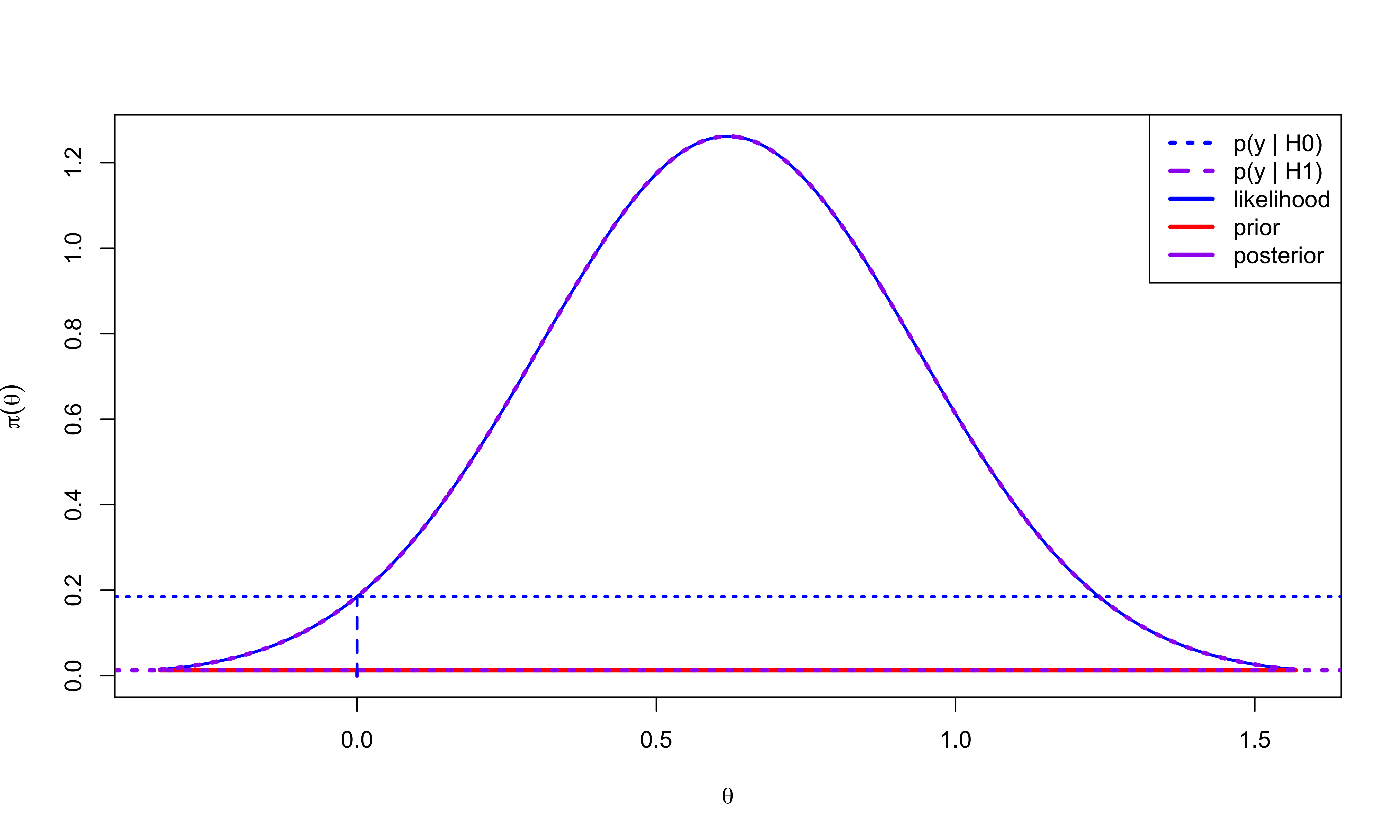
• \(\tau_0 = 1/1000\)

• Bayes Factor for \(\cal{H}_0\) to \(\cal{H}_1\) is \(14.65\)

• Posterior Probability of \(\cal{H}_0\) = 0.9361

Vague Priors & Hypothesis Testing

• As \(\tau_0 \to 0\) the \(\cal{BF}_{01} \to \infty\) and \(\Pr(\cal{H}_0 \mid \mathbf{y}\to 1\)!

• As we use a less & less informative prior for \(\theta\) under \(\cal{H}_1\) we obtain more & more evidence for \(\cal{H}_0\) over \(\cal{H}_1\)!

• Known as Bartlett’s Paradox - the paradox is that a seemingly non-informative prior for \(\theta\) is very informative about \(\cal{H}\)!

• General problem with nested sequence of models. If we choose vague priors on the additional parameter in the larger model we will be favoring the smaller models under consideration!

• Similar phenomenon with increasing sample size (Lindley’s Paradox)

Bottom Line Don’t use vague priors!

What should we use then?

Other Options

• Place a prior on \(\tau_0\) \[\tau_0 \sim \textsf{Gamma}(1/2, 1/2)\]

• If \(\theta \mid \tau_0, \cal{H}_1 \sim \textsf{N}(0, 1/\tau_0)\), then \(\theta_0 \mid \cal{H}_1\) has a \(\textsf{Cauchy}(0,1)\) distribution! Recommended by Jeffreys (1961)

• no closed form expressions for marginal likelihood!

Intrinsic Bayes Factors & Priors (Berger & Pericchi)

• Can’t use improper priors under \(\cal{H}_1\)

• use part of the data \(y(l)\) to update an improper prior on \(\theta\) to get a proper posterior \(\pi(\theta \mid \cal{H}_i, y(l))\)

• use \(\pi(\theta \mid y(l), \cal{H}_i)\) to obtain the posterior for \(\theta\) based on the rest of the training data

• Calculate a Bayes Factor (avoids arbitrary normalizing constants!)

• Choice of training sample \(y(l)\)?

• Berger & Pericchi (1996) propose “averaging” over training samples intrinsic Bayes Factors

• intrinsic prior on \(\theta\) that leads to the Intrisic Bayes Factor