Lecture 9: Gibbs Sampling and Data Augmentation

STA702

Merlise Clyde

Duke University

Normal Linear Regression Example

Model \[\begin{align*} Y_i \mid \beta, \phi & \overset{ ind}{\sim} \textsf{N}(x_i^T\beta, 1/\phi) \\ Y \mid \beta, \phi & \sim \textsf{N}(X \beta, \phi^{-1} I_n) \\ \beta & \sim \textsf{N}(b_0, \Phi_0^{-1}) \\ \phi & \sim \textsf{Gamma}(v_0/2, s_0/2) \end{align*}\]
\(x_i\) is a \(p \times 1\) vector of predictors and \(X\) is \(n \times p\) matrix
\(\beta\) is a \(p \times 1\) vector of coefficients
\(\Phi_0\) is a \(p \times p\) prior precision matrix
Multivariate Normal density for \(\beta\) \[\pi(\beta \mid b_0, \Phi_0) = \frac{|\Phi_0|^{1/2}}{(2 \pi)^{p/2}}\exp\left\{- \frac{1}{2}(\beta - b_0)^T \Phi_0 (\beta - b_0) \right\}\]

Full Conditional for \(\beta\)

\[\begin{align*} \beta & \mid \phi, y_1, \ldots, y_n \sim \textsf{N}(b_n, \Phi_n^{-1}) \\ b_n & = (\Phi_0 + \phi X^TX)^{-1}(\Phi_0 b_0 + \phi X^TX \hat{\beta})\\ \Phi_n & = \Phi_0 + \phi X^TX \end{align*}\]

Derivation continued

Full Conditional for \(\phi\)

\[\phi \mid \beta, y_1, \ldots, y_n \sim \textsf{Gamma}\left(\frac{v_0 + n}{2}, \frac{s_0 + \sum_i(y_i - x^T_i \beta)^2}{2}\right)\]

Choice of Prior Precision

Non-Informative \(\Phi_0 \to 0\)
Formal Posterior given \(\phi\) \[\beta \mid \phi, y_1, \ldots, y_n \sim \textsf{N}(\hat{\beta}, \phi^{-1} (X^TX)^{-1})\]
needs \(X^TX\) to be full rank for distribution to be unique!

Binary Regression

\[Y_i \mid \beta \sim \textsf{Ber}(p(x_i^T \beta))\] where \(\Pr(Y_i = 1 \mid \beta) = p(x_i^T \beta))\) and linear predictor \(x_i^T\beta = \lambda_i\)

link function for binary regression is any 1-1 function \(g\) that will map \((0,1) \to \mathbb{R}\), i.e. \(g(p(\lambda)) = \lambda\)
logistic regression uses the logit link
\[\log\left(\frac{p(\lambda_i)}{1 - p(\lambda_i) }\right) = x_i^T \beta = \lambda_i\]
probit link \[p(x_i^T \beta) = \Phi(x_i^T \beta)\]
\(\Phi()\) is the Normal cdf

Likelihood and Posterior

Likelihood: \[\cal{L}(\beta) \propto \prod_{i = 1}^n \Phi(x_i^T \beta)^{y_i} (1 - \Phi(x^T_i \beta))^{1 - y_i}\]

prior \(\beta \sim \textsf{N}_p(b_0, \Phi_0)\)
posterior \(\pi(\beta) \propto \pi(\beta) \cal{L}(\beta)\)
How to approximate the posterior?
- asymptotic Normal approximation
- MH with Independence chain or adaptive Metropolis
- stan (Hamiltonian Monte Carlo)
- Gibbs ?
seemingly no, but there is a trick!

Data Augmentation

Consider an augmented posterior \[\pi(\beta, Z \mid y) \propto \pi(\beta) \pi(Z \mid \beta) \pi(y \mid Z, \beta)\]
IF we choose \(\pi(Z \mid \beta)\) and \(\pi(y \mid Z, \beta)\) carefully, we can carry out Gibbs and get samples of \(\pi(\beta \mid y)\) !
desired marginal of joint augmented posterior \[\pi(\beta \mid y) = \int_{\cal{Z}} \pi(\beta, z \mid y) \, dz\]
We have to choose latent prior and sampling model such that \[p(y \mid \beta) = \int_{\cal{Z}} \pi(z \mid \beta) \pi(y \mid \beta, z) \, dz\]
complete data likelihood \(\pi(z \mid \beta) \pi(y \mid \beta, z)\)

Augmentation Strategy

Set

\(y_i = 1_{(Z_i > 0)}\) i.e. ( \(y_i = 1\) if \(Z_i > 0\) )
\(y_i = 1_{(Z_i < 0)}\) i.e. ( \(y_i = 0\) if \(Z_i < 0\) )
\(Z_i = x_i^T \beta + \epsilon_i \qquad \epsilon_i \overset{iid}{\sim} \textsf{N(0,1)}\)
Relationship to probit model: \[\begin{align*}\Pr(y = 1 \mid \beta) & = P(Z_i > 0 \mid \beta) \\ & = P(Z_i - x_i^T \beta > -x^T\beta) \\ & = P(\epsilon_i > -x^T\beta) \\ & = 1 - \Phi(-x^T_i \beta) \\ & = \Phi(x^T_i \beta) \end{align*}\]

Augmented Posterior & Gibbs

two block Gibbs sampler \(\theta_{[1]} = \beta\) and \(\theta_{[2]} = (Z_1, \ldots, Z_n)^T\) \[\begin{align*}\pi(& Z_1, \ldots, Z_n, \, \beta \mid y) \propto \\ & \textsf{N}(\beta; b_0, \phi_0) \left\{\prod_{i=1}^n \textsf{N}(Z_i; x_i^T\beta, 1)\right\} \left\{ \prod_{i=1}^n y_i 1_{(Z_i > 0)} + (1 - y_i)1_{(Z_i < 0)}\right\} \end{align*}\]
full conditional for \(\beta\) given \(Z_i\)’s based on Normal-Normal regression \[\beta \mid Z_1, \ldots, Z_n, y_1, \ldots, y_n \sim \textsf{N}(b_n, \Phi_n)\]
Full conditional for latent \(Z_i\) (product of independent dist’s) \[\begin{align*} \pi(Z_i \mid \beta, Z_{[-i]}, y_1, \ldots, y_n) & \propto \textsf{N}(Z_i; x_i^T \beta, 1)1_{(Z_i > 0)} \text{ if } y_1 = 1 \\ \pi(Z_i \mid \beta, Z_{[-i]}, y_1, \ldots, y_n) & \propto \textsf{N}(Z_i; x_i^T \beta, 1)1_{(Z_i < 0) }\text{ if } y_1 = 0 \\ \end{align*}\]

Truncated Sampling

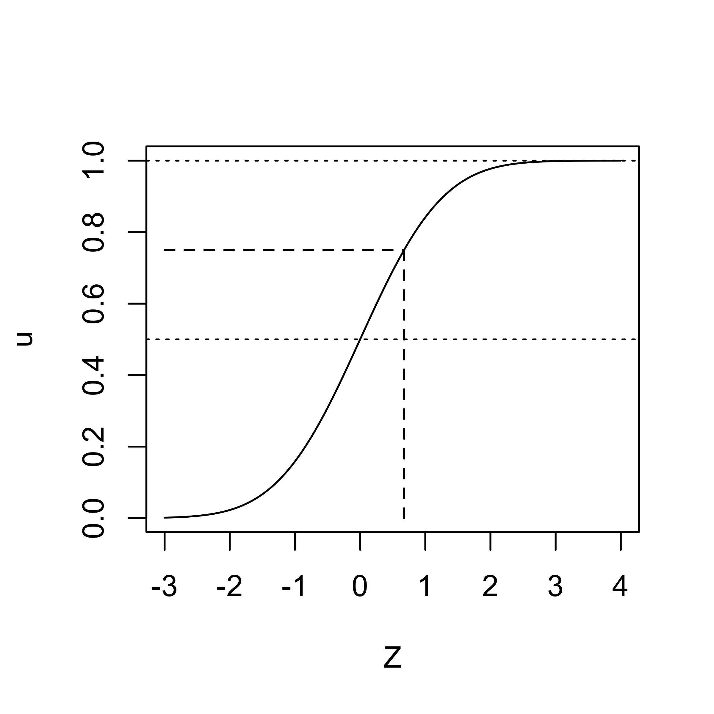
Use inverse cdf method for cdf \(F\)
If \(U\sim U(0,1)\) set \(X = F^{-1}(U)\)
if \(X \in (a, b)\), Draw \(X \sim U(F(a),F(b))\) and set \(X = F^{-1}(u)\)

Truncated Normal Sampling

sample from independent truncated normal distributions for full conditional for \(Z_i\)
if \(Y_i = 1\) then \(Z_i \sim \textsf{Normal}(x_i^T\beta, 1) I(0, \infty)\)
standard truncated normal \(\tilde{Z} = Z_i - x_i^T \beta \in (-x_i^T \beta, \infty)\)

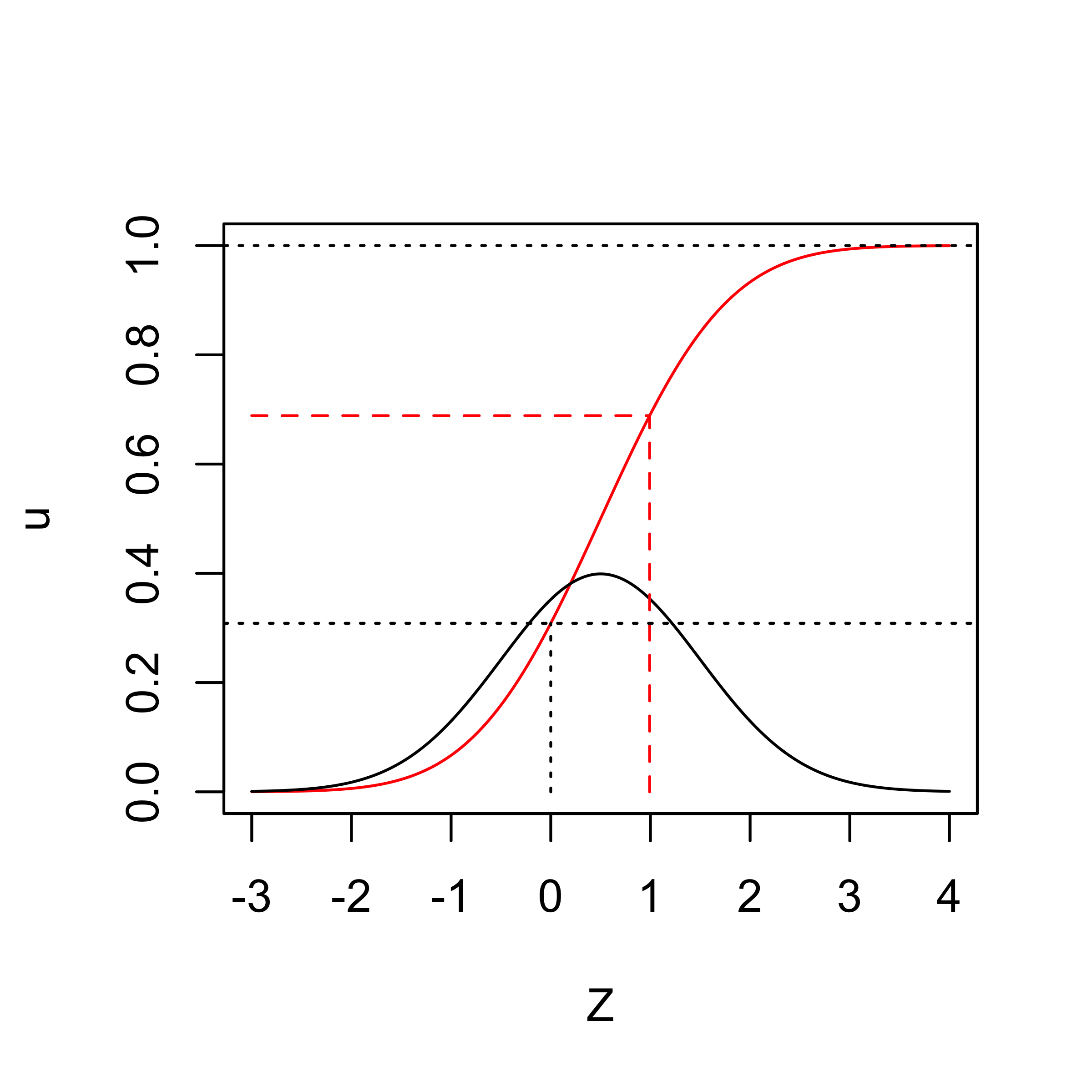
Generate \(U \sim \textsf{Uniform}(\Phi(-x_i^T\beta), \Phi(\infty))\)
Set \(\tilde{z} = \Phi^{-1}(U)\) (Standard truncated normal)
Shift \(Z_i = x_i^T \beta + \tilde{z}\)

U = 0.69, \(Z_i = x_i^T \beta + \Phi^{-1}(U)\) = 0.99

Comments on Gibbs

Why don’t we treat each individual \(\theta_j\) as a separate block?
Gibbs always accepts, but can mix slowly if parameters in different blocks are highly correlated!
Use block sizes in Gibbs that are as big as possible to improve mixing (proven faster convergence)
Collapse the sampler by integrating out as many parameters as possible (as long as resulting sampler has good mixing)
can use Gibbs steps and (adaptive) Metropolis Hastings steps together
latent variables may allow Gibbs steps, but not always better compared to MH!

Data Augmentation in General

DA is a broader than a computational trick allowing Gibbs sampling

random effects or latent variable modeling i.e we introduce latent variables to simplify dependence structure modelling
Modeling heavy tailed distributions for priors or errors in robust regression as mixtures of normals
outliers
variable selection
missing data
Next class:
- Multivariate Normal data
- Wishart and inverse-Wishart distributions
- missing data