Lecture 7: MCMC Diagnostics & Adaptive Metropolis

STA702

Merlise Clyde

Duke University

Example from Last Class

Marginal Likelihood \[\cal{L}(\mu, \sigma^2, \sigma^2_\mu) \propto (\sigma^2 + \sigma^2_\mu)^{-n/2} \exp \left\{ - \frac{1}{2} \frac{\sum_{i=1}^n\left(y_i - \mu \right)^2}{\sigma^2 + \sigma^2_\mu }\right\}\]
Priors with \(\sigma^2 = 1\): \(p(\mu) \propto 1\) and \(\sigma_\mu \sim \textsf{Cauchy}^+(0,1)\) independent of \(\mu\)
Symmetric proposal for \(\mu\) and \(\sigma_\tau\)
Independent normals centered at current values of \(\mu\) and \(\sigma_\mu\) with covariance \(\frac{2.38^2}{d} \textsf{Cov}(\theta)\) where \(d = 2\) (the dimension of \(\theta\) )
\(\delta^2 = 2.38^2/d\) optimal for multivariate normal target Roberts, Gelman, and Gilks (1997) with acceptance rate ranging from 40% to 23.4% (as \(d \to \infty\))

Convergence diagnostics

Diagnostics available to help decide on number of burn-in & collected samples.
Note: no definitive tests of convergence but you should do as many diagnostics as you can, on all parameters in your model.
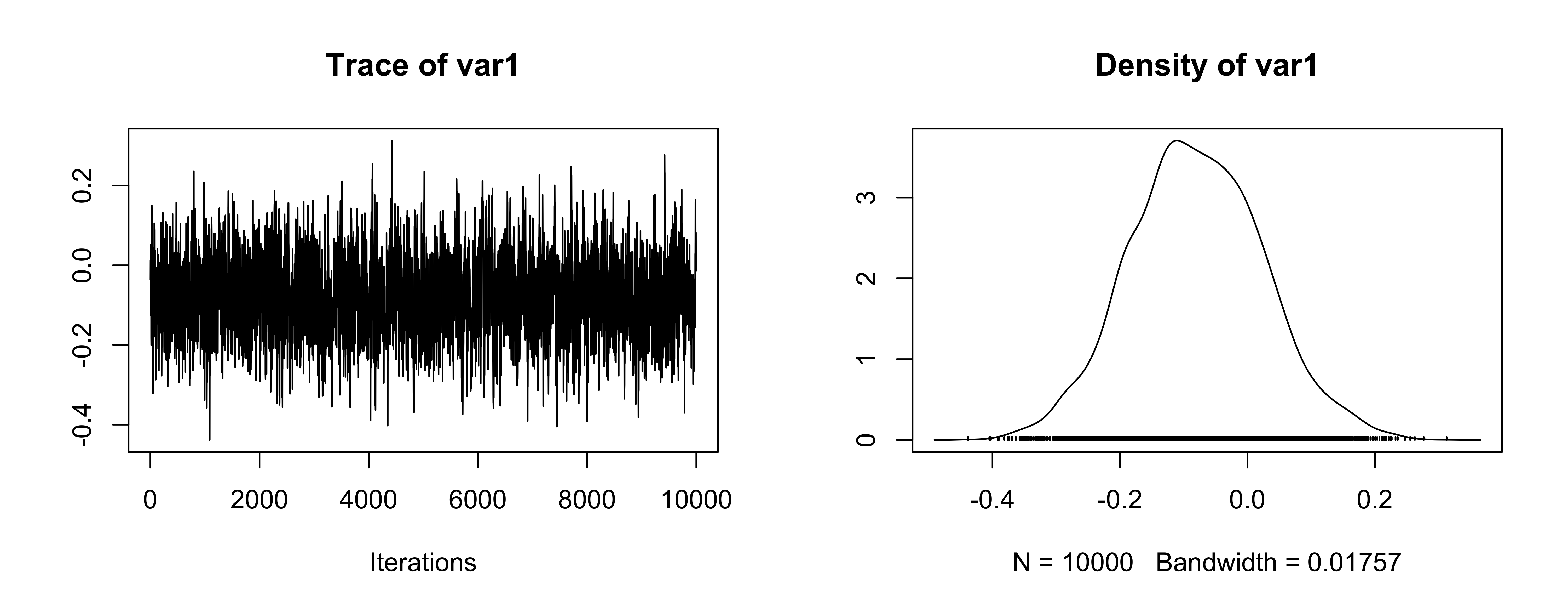
With “experience”, visual inspection of trace plots perhaps most useful approach.
There are a number of useful automated tests in R.
CAUTION: diagnostics cannot guarantee that a chain has converged, but they can indicate it has not converged.

Diagnostics in R

The most popular package for MCMC diagnostics in R is coda.
coda uses a special MCMC format so you must always convert your posterior matrix into an MCMC object.
For the example, we have the following in R.

#library(coda)
theta.mcmc <- mcmc(theta,start=1) #no burn-in (simple problem!)

Diagnostics in R

summary(theta.mcmc)


Iterations = 1:10000
Thinning interval = 1 
Number of chains = 1 
Sample size per chain = 10000 

1. Empirical mean and standard deviation for each variable,
   plus standard error of the mean:

             Mean     SD Naive SE Time-series SE
mu       -0.07977 0.1046 0.001046       0.002839
sigma_mu  0.17550 0.1273 0.001273       0.004397

2. Quantiles for each variable:

              2.5%     25%      50%      75%  97.5%
mu       -0.283420 -0.1508 -0.08193 -0.00848 0.1337
sigma_mu  0.007995  0.0758  0.15024  0.25228 0.4693

The naive SE is the standard error of the mean, which captures simulation error of the mean rather than the posterior uncertainty.
The time-series SE adjusts the naive SE for autocorrelation.

Effective Sample Size

The effective sample size translates the number of MCMC samples \(S\) into an equivalent number of independent samples.
It is defined as \[\textrm{ESS} = \dfrac{S}{1 + 2 \sum_k \rho_k},\]
\(S\) is the sample size and \(\rho_k\) is the lag \(k\) autocorrelation.
For our data, we have

effectiveSize(theta.mcmc)

       mu  sigma_mu 
1356.6495  838.2613

So our 10,000 samples are equivalent to 1356.6 independent samples for \(\mu\) and 838.3 independent samples for \(\sigma_\mu\).

Trace plot for mean

Trace plot for \(\sigma_\mu\)

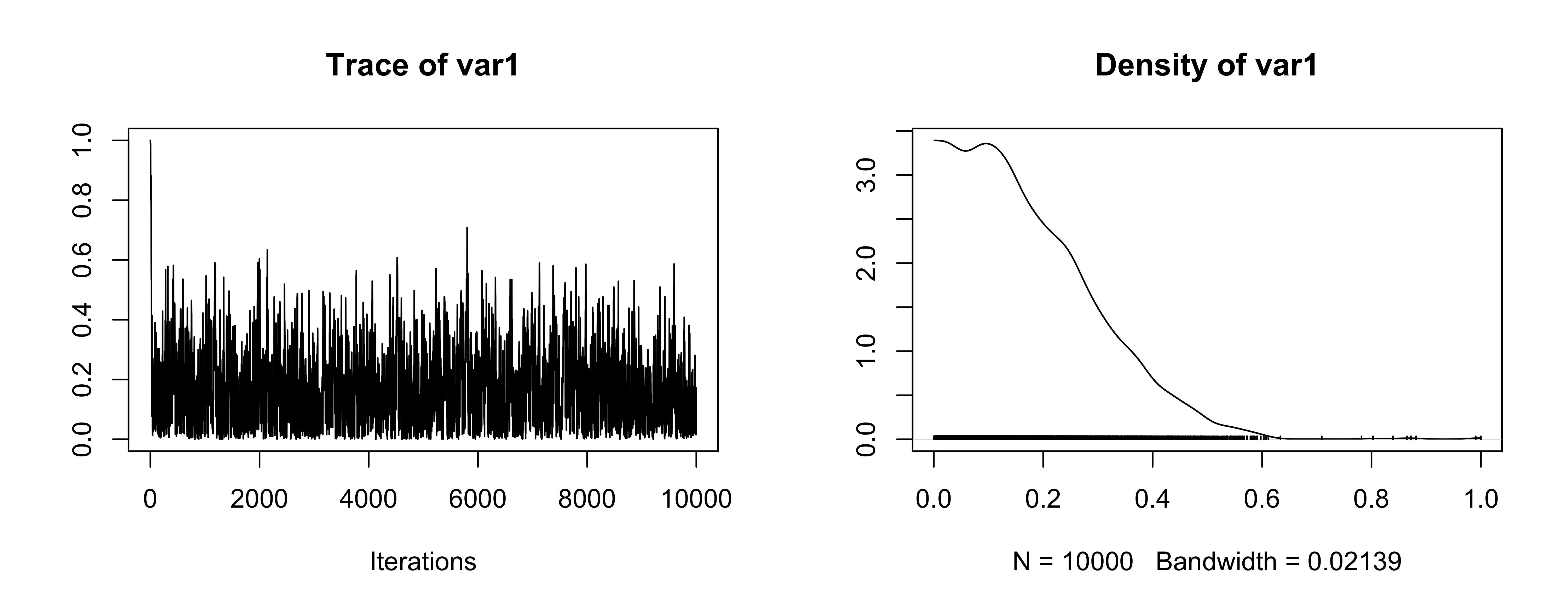
OK (be careful of scaling in plots!)

Autocorrelation

Another way to evaluate convergence is to look at the autocorrelation between draws of our Markov chain.
The lag \(k\) autocorrelation, \(\rho_k\), is the correlation between each draw and its \(k\)th lag, defined as \[\rho_k = \dfrac{\sum_{s=1}^{S-k}(\theta_s - \bar{\theta})(\theta_{s+k} - \bar{\theta})}{\sum_{s=1}^{S-k}(\theta_s - \bar{\theta})^2}\]
We expect the autocorrelation to decrease as \(k\) increases.
If autocorrelation remains high as \(k\) increases, we have slow mixing due to the inability of the sampler to move around the space well.

Autocorrelation for mean

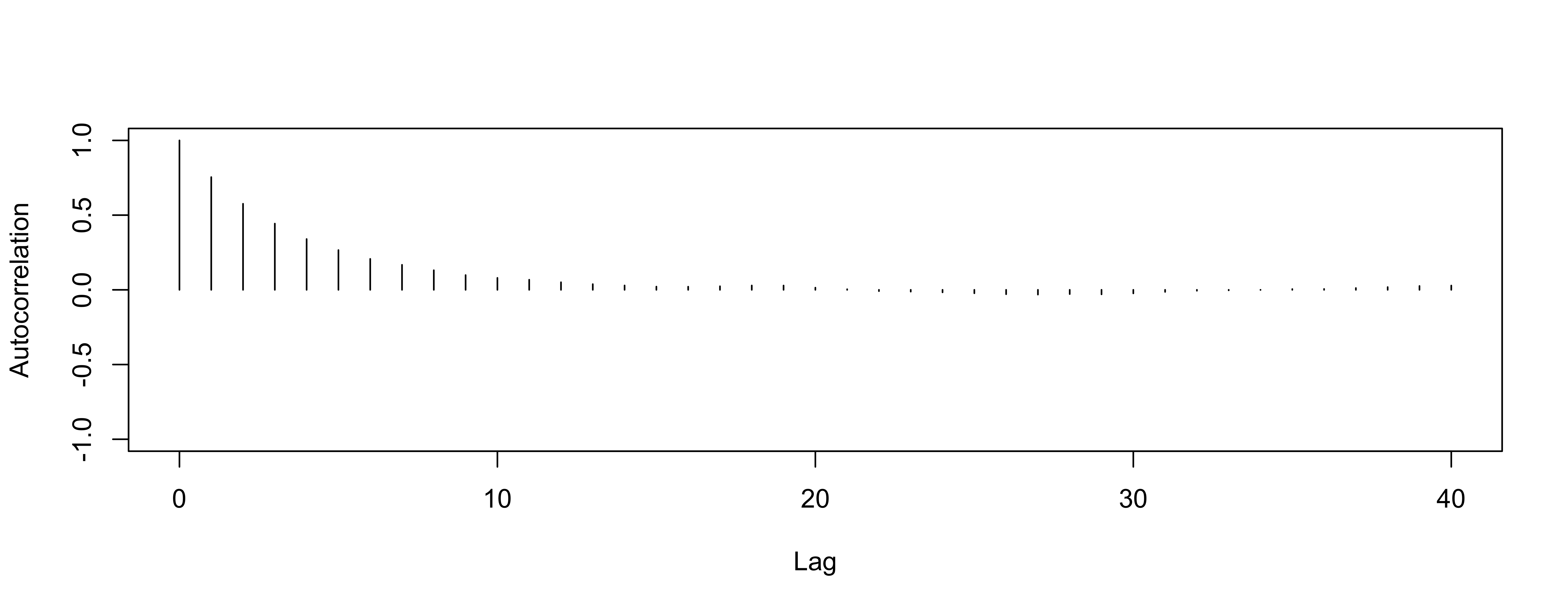
So-So

Autocorrelation for variance

worse

Gelman-Rubin

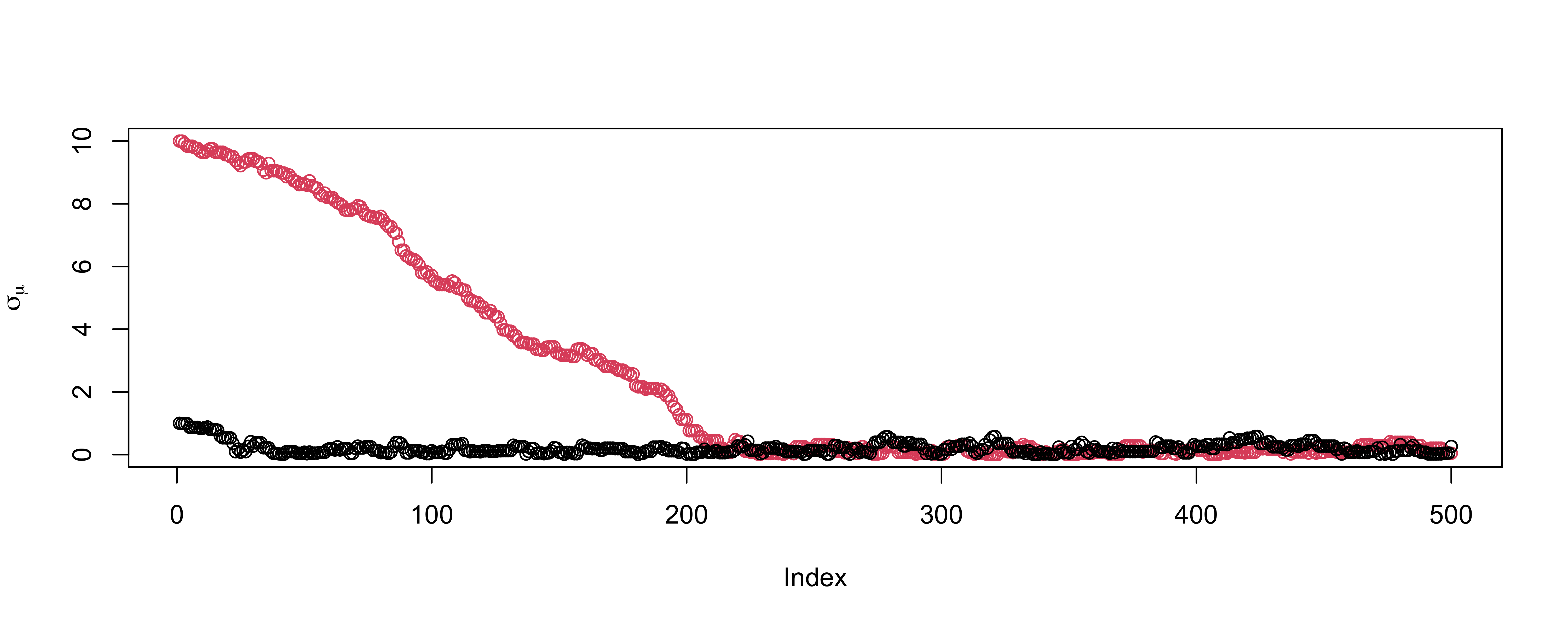
Gelman & Rubin suggested a diagnostic \(R\) based on taking separate chains with dispersed initial values to test convergence

Gelman-Rubin Diagnostic

Run m > 2 chains of length 2S from overdispersed starting values.
Discard the first S draws in each chain.
Calculate the pooled within-chain variance \(W\) and between-chain variance \(B\). \[R = \frac{\frac{S-1}{S} W + \frac{1}{S} B }{W}\]
numerator and denominator are both unbiased estimates of the variance if the two chains have converged
- otherwise \(W\) is an underestimate (hasn’t explored enough)
- numerator will overestimate as \(B\) is too large (overdispersed starting points)
As \(S \to \infty\) and \(B \to 0\), \(R \to 1\)
version in R is slightly different

Gelman-Rubin Diagnostic

theta.mcmc = mcmc.list(mcmc(theta1, start=5000), mcmc(theta2, start=5000))
gelman.diag(theta.mcmc)

Potential scale reduction factors:

         Point est. Upper C.I.
mu                1          1
sigma_mu          1          1

Multivariate psrf

1

Values of \(R > 1.1\) suggest lack of convergence
Looks OK
See also gelman.plot

Geweke statistic

Geweke proposed taking two non-overlapping parts of a single Markov chain (usually the first 10% and the last 50%) and comparing the mean of both parts, using a difference of means test
The null hypothesis would be that the two parts of the chain are from the same distribution.
The test statistic is a z-score with standard errors adjusted for autocorrelation, and if the p-value is significant for a variable, you need more draws.
Output in R is the Z score

Geweke Diagnostic

geweke.diag(theta.mcmc)

[[1]]

Fraction in 1st window = 0.1
Fraction in 2nd window = 0.5 

      mu sigma_mu 
 -0.7779   0.7491 


[[2]]

Fraction in 1st window = 0.1
Fraction in 2nd window = 0.5 

      mu sigma_mu 
  0.4454   0.6377

The output is the z-score itself (not the p-value).

Practical advice on diagnostics

There are more tests we can use: Raftery and Lewis diagnostic, Heidelberger and Welch, etc.
The Gelman-Rubin approach is quite appealing in using multiple chains
Geweke (and Heidelberger and Welch) sometimes reject even when the trace plots look good.
Overly sensitive to minor departures from stationarity that do not impact inferences.
Most common method of assessing convergence is visual examination of trace plots.

Improving Results

more iterations and multiple chains
thinning to reduce correlations and increase ESS
change the proposal distribution \(q\)
adaptive Metropolis to tune \(q\)

Proposal Distribution

Common choice \[\textsf{N}(\theta^\star; \theta^{(s)}, \delta^2 \Sigma)\]
rough estimate of \(\Sigma\) based on the asymptotic Gaussian approximation \(\textsf{Cov}(\theta \mid y)\) and \(\delta = 2.38/\sqrt{\text{dim}(\theta)}\)
find the MAP estimate (posterior mode) \(\hat{\theta}\)
take \[\Sigma = \left[- \frac{\partial^2 \log(\cal{L}(\theta)) + \log(\pi(\theta))} {\partial \theta \partial \theta^T} \right]^{-1}_{\theta = \hat{\theta}}\]
ignore prior and use inverse of Fisher Information (covariance of MLE)

Learn Covariance in Proposal?

Can we learn the proposal distribution?
ad hoc?
- run an initial MCMC for an initial tuning phase (e.g. 1000 samples) with a fixed \(\delta\) and estimate \(\Sigma(\theta)\) from samples.
- run more to tweak \(\delta\) to get acceptance rate between \(23\%-40\%\).
- fix the kernel for final run
MCMC doesn’t allow you to use the full history of the chain \(\theta^{(1)}, \ldots, \theta^{(s)}\) in constructing the proposal distributions as it violates the Markov assumption
even with no further “learning”, no guarantee we will converge to posterior!
more elegant approach - formal adaptive Metropolis
- keep adapting the entire time!

ad hoc adaptation may mess up convergence !

Adaptive MCMC

run RWM with a Gaussian proposal for a fixed number of iterations for \(s < s_0\)
estimate of covariance at state \(s\) \[\Sigma^{(s)} = \frac{1}{s}\left(\sum_{i=1}^s \theta^{(i)} {\theta^{(i)}}^T - s \bar{\theta}^{(s)} {\bar{\theta}^{(s)}}^T\right)\]
proposal for \(s > s_0\) with \(\delta = 2.38/\sqrt{d}\) \[\theta^* \sim \textsf{N}(\theta^{(s)}, \delta^2 (\Sigma^{(s)} + \epsilon I_d))\]
\(\epsilon > 0\) insures covariance is positive definite
if \(s_0\) is too large will take longer for adaptation to be seen
need conditions for vanishing adaptation e.g. that the proposal depends less and less on recent states in the chain - see Roberts & Rosenthal (2009)for examples and other conditions

Example again

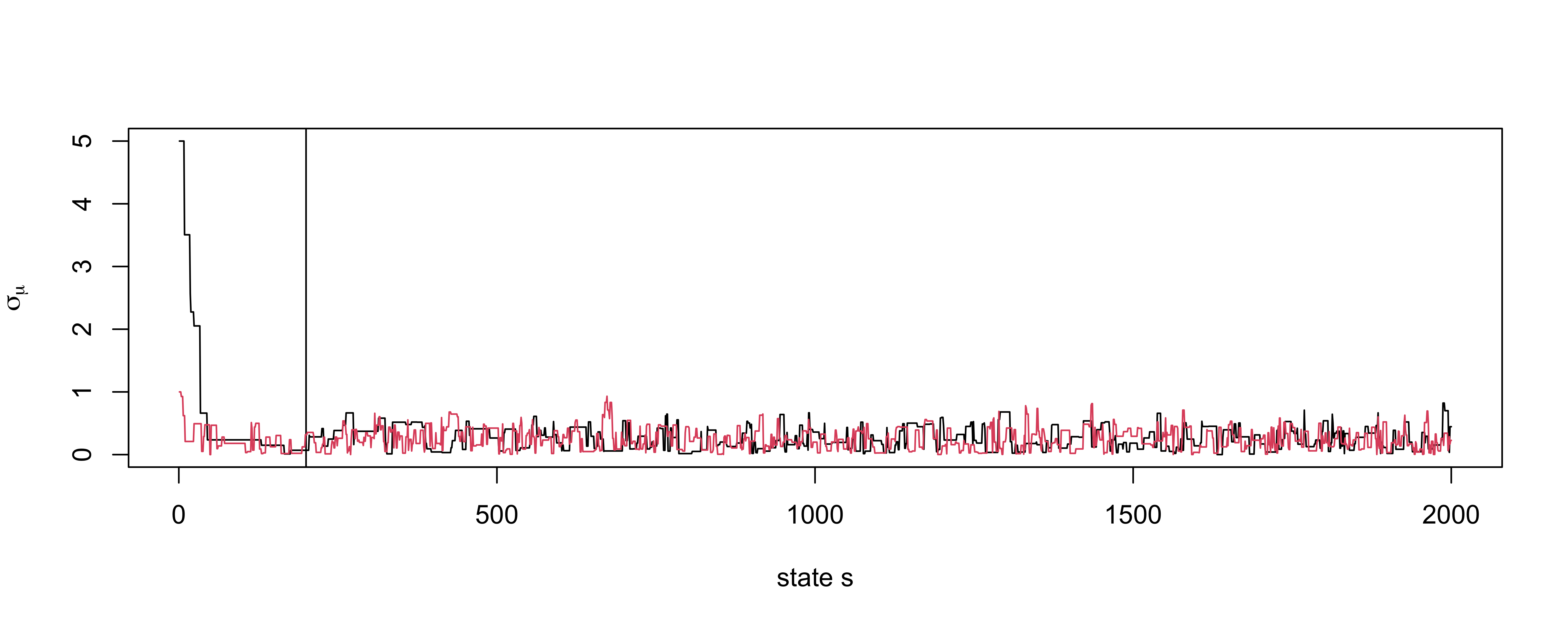
Acceptance rate now around 30-35 % of 10,000 iterations!