Introduction to Hierarchical Modelling, Empirical Bayes, and MCMC

STA702 Lecture 5

Merlise Clyde

Duke University

Normal Means Model

Suppose we have normal data with \[Y_i \mid \mu_i, \sigma^2 \overset{ind}{\sim} \textsf{N}(\mu_i, \sigma^2)\]
separate mean for each observation!
Question: How can we possibly hope to estimate all these \(\mu_i\)? One \(y_i\) per \(\mu_i\) and \(n\) observations!
Naive estimator: just consider only using \(y_i\) in estimating and not the other observations.
MLE \(\hat{\mu}_i = y_i\)
Hierarchical Viewpoint: Let’s borrow information from other observations!

Motivation

Example \(y_i\) is difference in gene expression for the \(i^{\text{th}}\) gene between cancer and control lines
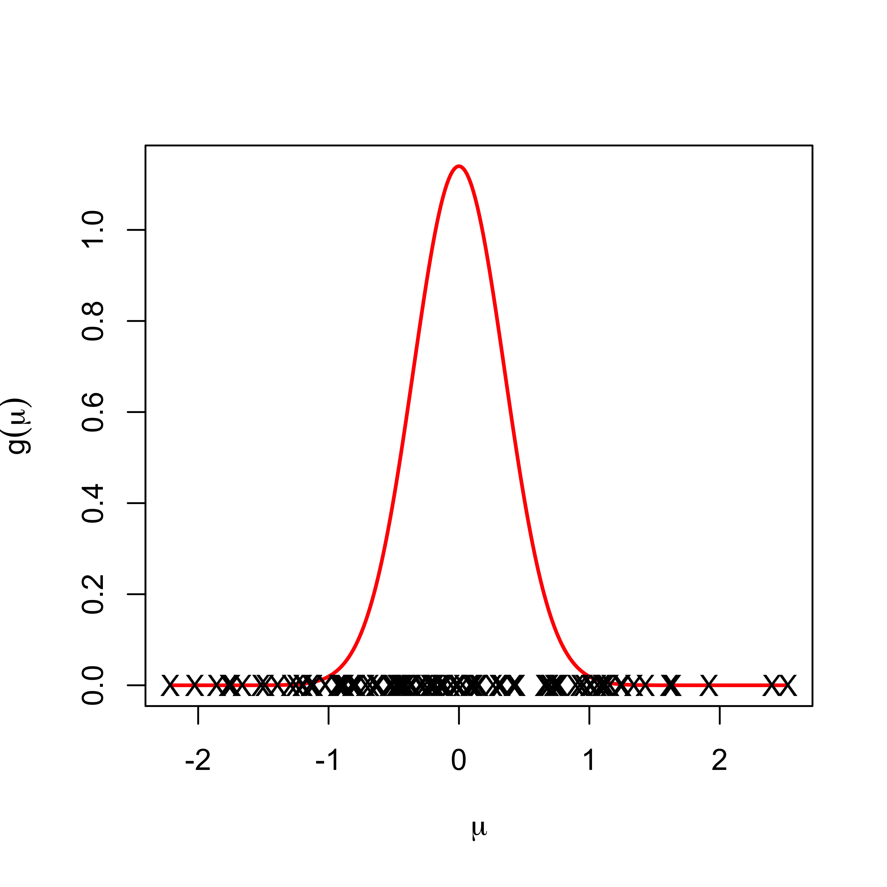
may be natural to think that the \(\mu_i\) arise from some common distribution, \(\mu_i \overset{iid}{\sim} g\)
unbiased but high variance estimators of \(\mu_i\) based on one observation!

Low Variability

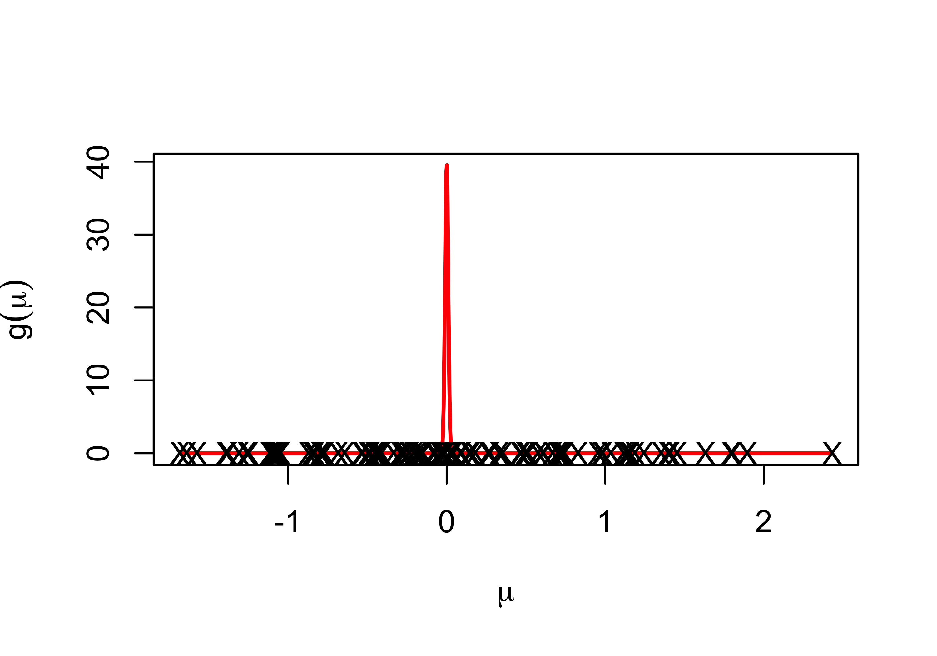
little variation in \(\mu_i\)s so a better estimate might be \(\bar{y}\)
Not forced to choose either - what about some weighted average between \(y_i\) and \(\bar{y}\)?

Simple Example

Data Model \[Y_i \mid \mu_i, \sigma^2 \overset{ind}{\sim} \textsf{N}(\mu_i, \sigma^2)\]
Means Model \[\mu_i \mid \mu, \sigma^2_\mu \overset{iid}{\sim} \textsf{N}(\mu, \sigma^2_{\mu})\]
not necessarily a prior!
Now estimate \(\mu_i\) (let \(\phi = 1/\sigma^2\) and \(\phi_{\mu} = 1/\sigma^2_\mu\))
Calculate the “posterior” \(\mu_i \mid y_i, \mu, \phi, \phi_\mu\)

Hiearchical Estimates

Posterior: \(\mu_i \mid y_i, \mu, \phi, \phi_\mu \overset{ind}{\sim} \textsf{N}(\tilde{\mu}_i, 1/\tilde{\phi}_\mu)\)
estimator of \(\mu_i\) weighted average of data and population parameter \(\mu\) \[\tilde{\mu}_i = \frac{\phi_\mu \mu + \phi y_i} {\phi_\mu + \phi} \qquad \qquad \tilde{\phi}_\mu = \phi + \phi_\mu\]
if \(\phi_\mu\) is large relative to \(\phi\) all of the \(\mu_i\) are close together and benefit by borrowing information
in limit as \(\sigma^2_\mu \to 0\) or \(\phi_\mu \to \infty\) we have \(\tilde{\mu}_i = \mu\) (all means are the same)
if \(\phi_\mu\) is small relative to \(\phi\) little borrowing of information
in the limit as \(\phi_\mu \to 0\) we have \(\tilde{\mu}_i = y_i\)

Bayes Estimators and Bias

Note: you often benefit from a hierarchical model, even if its not obvious that the \(\mu_i\) are related!
The MLE for the \(\mu_i\) is just the sample \(y_i\).
\(y_i\) is unbiased for \(\mu_i\) but can have high variability!
the posterior mean is actually biased.
Usually through the weighting of the sample data and prior, Bayes procedures have the tendency to pull the estimate of \(\mu_i\) toward the prior or provide shrinkage to the mean.

Question

Why would we ever want to do this? Why not just stick with the MLE?

MSE or Bias-Variance Tradeoff

Modern Relevance

The fact that a biased estimator would do a better job in many estimation/prediction problems can be proven rigorously, and is referred to as Stein’s paradox.
Stein’s result implies, in particular, that the sample mean is an inadmissible estimator of the mean of a multivariate normal distribution in more than two dimensions i.e. there are other estimators that will come closer to the true value in expectation.
In fact, these are Bayes point estimators (the posterior expectation of the parameter \(\mu_i\)).
Most of what we do now in high-dimensional statistics is develop biased estimators that perform better than unbiased ones.
Examples: lasso regression, ridge regression, various kinds of hierarchical Bayesian models, etc.

Population Parameters

we don’t know \(\mu\) (or \(\sigma^2\) and \(\sigma^2_\mu\) for that matter)
Find marginal likelihood \(\cal{L}(\mu, \sigma^2, \sigma^2_\mu)\) by integrating out \(\mu_i\) with respect to \(g\) \[\cal{L}(\mu, \sigma^2, \sigma^2_\mu) \propto \prod_{i = 1}^n \int \textsf{N}(y_i; \mu_i, \sigma^2) \textsf{N}(\mu_i; \mu, \sigma^2_\mu) \, d \mu_i\]
Product of predictive distributions for \(Y_i \mid \mu, \sigma^2, \sigma^2_\mu \overset{iid}{\sim} \textsf{N}(\mu, \sigma^2 + \sigma^2_\mu)\)
\[\cal{L}(\mu, \sigma^2, \sigma^2_\mu) \propto \prod_{i = 1}^n (\sigma^2 + \sigma^2_\mu)^{-1/2} \exp \left\{ - \frac{1}{2} \frac{\left(y_i - \mu \right)^2}{\sigma^2 + \sigma^2_\mu }\right\}\]
Find MLE’s

MLEs

\[\cal{L}(\mu, \sigma^2, \sigma^2_\mu) \propto (\sigma^2 + \sigma^2_\mu)^{-n/2} \exp\left\{ - \frac{1}{2} \sum_{i=1}^n\frac{\left(y_i - \mu \right)^2}{\sigma^2 + \sigma^2_\mu }\right\}\]

MLE of \(\mu\): \(\hat{\mu} = \bar{y}\)
Can we say anything about \(\sigma^2_\mu\)? or \(\sigma^2\) individually?
MLE of \(\sigma^2 + \sigma^2_\mu\) is \[\widehat{\sigma^2 + \sigma^2_\mu} = \frac{\sum(y_i - \bar{y})^2}{n}\]
Assume \(\sigma^2\) is known (say 1) \[\hat{\sigma}^2_\mu = \frac{\sum(y_i - \bar{y})^2}{n} - 1\]

Empirical Bayes Estimates

plug in estimates of hyperparameters into the prior and pretend they are known
resulting estimates are known as Empirical Bayes
Estimates of variances may be negative - constrain to 0 on the boundary
underestimates uncertainty
Fully Bayes would put a prior on the unknowns

Bayes and Hierarchical Models

We know the conditional posterior distribution of \(\mu_i\) given the other parameters, lets work with the marginal likelihood \(\cal{L}(\theta)\)
need a prior \(\pi(\theta)\) for unknown parameters are \(\theta = (\mu, \sigma^2, \sigma^2_\mu)\) (details later)
Posterior \[\pi(\theta \mid y) = \frac{\pi(\theta) \cal{L}(\theta)} {\int_\Theta \pi(\theta) \cal{L}(\theta) \, d\theta} = \frac{\pi(\theta) \cal{L}(\theta)} {m(y)}\]
Problems: Except for simple cases (conjugate models) \(m(y)\) is not available analytically

Large Sample Approximations

Appeal to BvM (Bayesian Central Limit Theorem) and approximate \(\pi(\theta \mid y)\) with a Gaussian distribution centered at the posterior mode \(\hat{\theta}\) and asymptotic covariance matrix \[V_\theta = \left[- \frac{\partial^2}{\partial \theta \partial \theta^T} \left\{\log(\pi(\theta)) + \log(\cal{L}(\theta)) \right\} \right]^{-1}\]
related to Laplace approximation to integral (also large sample)
Use normal approximation to find \(\textsf{E}[h(\theta) \mid y]\)
Integral may not exist in closed form (non-linear functions)
use numerical quadrature (doesn’t scale up)
Stochastic methods of integration

Stochastic Integration

Stochastic integration \[\textsf{E}[h(\theta) \mid y] = \int_\Theta h(\theta) \pi(\theta \mid y) \, d\theta \approx \frac{1}{T}\sum_{t=1}^{T} h(\theta^{(t)}) \qquad \theta^{(t)} \sim \pi(\theta \mid y)\]
what if we can’t sample from the \(\pi(\theta \mid y)\) but can sample from some distribution \(q()\) \[\textsf{E}[h(\theta) \mid y] = \int_\Theta h(\theta) \frac{\pi(\theta \mid y)}{q(\theta)} q(\theta)\, d\theta \approx \frac{1}{T}\sum_{t=1}^{T} h(\theta^{(t)}) \frac{\pi(\theta^{(t)} \mid y)} {q(\theta^{(t)})} \qquad\] where \(\theta^{(t)} \sim q(\theta)\)
Without the \(m(y)\) in \(\pi(\theta \mid y)\) we just have \(\pi(\theta \mid y) \propto \pi(\theta) \cal{L}(\theta)\)
use twice for numerator and denominator

Important Sampling Estimate

Estimate of \(m(y)\) \[m(y) \approx \frac{1}{T} \sum_{t=1}^{T} \frac{\pi(\theta^{(t)}) \cal{L}(\theta^{(t)})}{q(\theta^{(t)})} \qquad \theta^{(t)} \sim q(\theta)\]
Ratio estimator of \(\textsf{E}[h(\theta) \mid y]\) \[\textsf{E}[h(\theta) \mid y] \approx \frac{\sum_{t=1}^{T} h(\theta^{(t)}) \frac{\pi(\theta^{(t)}) \cal{L}(\theta^{(t)})}{q(\theta^{(t)})}} { \sum_{t=1}^{T} \frac{\pi(\theta^{(t)}) \cal{L}(\theta^{(t)})}{q(\theta^{(t)})}} \qquad \theta^{(t)} \sim q(\theta)\]
Weighted average with importance weights \(w(\theta^{(t)}) \propto \frac{\pi(\theta^{(t)}) \cal{L}(\theta^{(t)})}{q(\theta^{(t)})}\) \[\textsf{E}[h(\theta) \mid y] \approx \sum_{t=1}^{T} h(\theta^{(t)}) w(\theta^{(t)})/\sum_{t=1}^T w(\theta^{(t)}) \qquad \theta^{(t)} \sim q(\theta)\]

Issues

if \(q()\) puts too little mass in regions with high posterior density, we can have some extreme weights
optimal case is that \(q()\) is as close as possible to the posterior so that all weights are constant
Estimate may have large variance
Problems with finding a good \(q()\) in high dimensions \((d > 20)\) or with skewed distributions

Markov Chain Monte Carlo (MCMC)

Typically \(\pi(\theta)\) and \(\cal{L}(\theta)\) are easy to evaluate

Question

How do we draw samples only using evaluations of the prior and likelihood in higher dimensional settings?

construct a Markov chain \(\theta^{(t)}\) in such a way the the stationary distribution of the Markov chain is the posterior distribution \(\pi(\theta \mid y)\)! \[\theta^{(0)} \overset{k}{\longrightarrow} \theta^{(1)} \overset{k}{\longrightarrow} \theta^{(2)} \cdots\]
\(k_t(\theta^{(t-1)} ; \theta^{(t)})\) transition kernel
initial state \(\theta^{(0)}\)
choose some nice \(k_t\) such that \(\theta^{(t)} \to \pi(\theta \mid y)\) as \(t \to \infty\)
biased samples initially but get closer to the target
Metropolis Algorithm (1950’s)

Stochastic Sampling Intuition

From a sampling perspective, we need to have a large sample or group of values, \(\theta^{(1)}, \ldots, \theta^{(S)}\) from \(\pi(\theta \mid y)\) whose empirical distribution approximates \(\pi(\theta \mid y)\).
for any two sets \(A\) and \(B\), we want \[\frac{\dfrac{\# \theta^{(s)} \in A}{S}}{\dfrac{\# \theta^{(s)} \in B}{S} } = \dfrac{\# \theta^{(s)} \in A}{\# \theta^{(s)} \in B} \approx \dfrac{\pi(\theta \in A \mid y)}{\pi(\theta \in B \mid y)}\]
Suppose we have a working group \(\theta^{(1)}, \ldots, \theta^{(s)}\) at iteration \(s\), and need to add a new value \(\theta^{(s+1)}\).
Consider a candidate value \(\theta^\star\) that is close to \(\theta^{(s)}\)
Should we set \(\theta^{(s+1)} = \theta^\star\) or not?

Posterior Ratio.

look at the ratio \[ \begin{split} M & = \dfrac{\pi(\theta^\star \mid y)}{\pi(\theta^{(s)} \mid y)} = \frac{\dfrac{p(y \mid \theta^\star) \pi(\theta^\star)}{p(y)} } {\dfrac{p(y \mid \theta^{(s)}) \pi(\theta^{(s)})}{p(y)}}\\ \\ & = \dfrac{p(y \mid \theta^\star) \pi(\theta^\star)}{p(y \mid \theta^{(s)}) \pi(\theta^{(s)})} \end{split} \]

does not depend on the marginal likelihood we don’t know!

Metropolis algorithm

If \(M > 1\)
- Intuition: \(\theta^{(s)}\) is already a part of the density we desire and the density at \(\theta^\star\) is even higher than the density at \(\theta^{(s)}\).
- Action: set \(\theta^{(s+1)} = \theta^\star\)
If \(M < 1\),
- Intuition: relative frequency of values in our group \(\theta^{(1)}, \ldots, \theta^{(s)}\) “equal” to \(\theta^\star\) should be \(\approx M = \dfrac{\pi(\theta^\star \mid y)}{\pi(\theta^{(s)} \mid y)}\).
- For every \(\theta^{(s)}\), include only a fraction of an instance of \(\theta^\star\).
- Action: set \(\theta^{(s+1)} = \theta^\star\) with probability \(M\) and \(\theta^{(s+1)} = \theta^{(s)}\) with probability \(1-M\).

Proposal Distribution

Where should the proposed value \(\theta^\star\) come from?
Sample \(\theta^\star\) close to the current value \(\theta^{(s)}\) using a symmetric proposal distribution \(\theta^\star \sim q(\theta^\star \mid \theta^{(s)})\)
\(q()\) is actually a “family of proposal distributions”, indexed by the specific value of \(\theta^{(s)}\).
Here, symmetric means that \(q(\theta^\star \mid \theta^{(s)}) = q(\theta^{(s)} \mid \theta^\star)\).
Common choice \[\textsf{N}(\theta^\star; \theta^{(s)}, \delta^2 \Sigma)\] with \(\Sigma\) based on the approximate \(\textsf{Cov}(\theta \mid y)\) and \(\delta = 2.44/\text{dim}(\theta)\) or \[\text{Unif}(\theta^\star; \theta^{(s)} - \delta, \theta^{(s)} + \delta)\]

Metropolis Algorithm Recap

The algorithm proceeds as follows:

Given \(\theta^{(1)}, \ldots, \theta^{(s)}\), generate a candidate value \(\theta^\star \sim q(\theta^\star \mid \theta^{(s)})\).
Compute the acceptance ratio \[\begin{split} M & = \dfrac{\pi(\theta^\star \mid y)}{\pi(\theta^{(s)} \mid y)} = \dfrac{p(y \mid \theta^\star) \pi(\theta^\star)}{p(y \mid \theta^{(s)}) \pi(\theta^{(s)})}. \end{split}\]
Set \[\begin{eqnarray*} \theta^{(s+1)} = \left\{ \begin{array}{ll} \theta^\star & \quad \text{with probability} \quad \text{min}(M,1) \\ \theta^{(s)} & \quad \text{with probability} \quad 1 - \text{min}(M,1) \\ \end{array} \right. \end{eqnarray*}\] equivalent to sampling \(u \sim U(0,1)\) independently and setting \[\begin{eqnarray*} \theta^{(s+1)} = \left\{ \begin{array}{ll} \theta^\star & \quad \text{if} \quad u < M \\ \theta^{(s)} & \quad \text{if} \quad \text{otherwise} \\ \end{array} \right. . \end{eqnarray*} \]

Notes

Acceptance probability is \[M = \min \left\{ 1, \frac{\pi(\theta^\star) \cal{L}(\theta^\star)} {\pi(\theta^{(s)}) \cal{L}(\theta^{(s)})}\right\}\]
ratio of posterior densities where normalizing constant cancels!
The Metropolis chain ALWAYS moves to the proposed \(\theta^\star\) at iteration \(s+1\) if \(\theta^\star\) has higher target density than the current \(\theta^{(s)}\).
Sometimes, it also moves to a \(\theta^\star\) value with lower density in proportion to the density value itself.
This leads to a random, Markov process that naturally explores the space according to the probability defined by \(\pi(\theta \mid y)\), and hence generates a sequence that, while dependent, eventually represents draws from \(\pi(\theta \mid y)\) (stationary distribution of the Markov Chain).