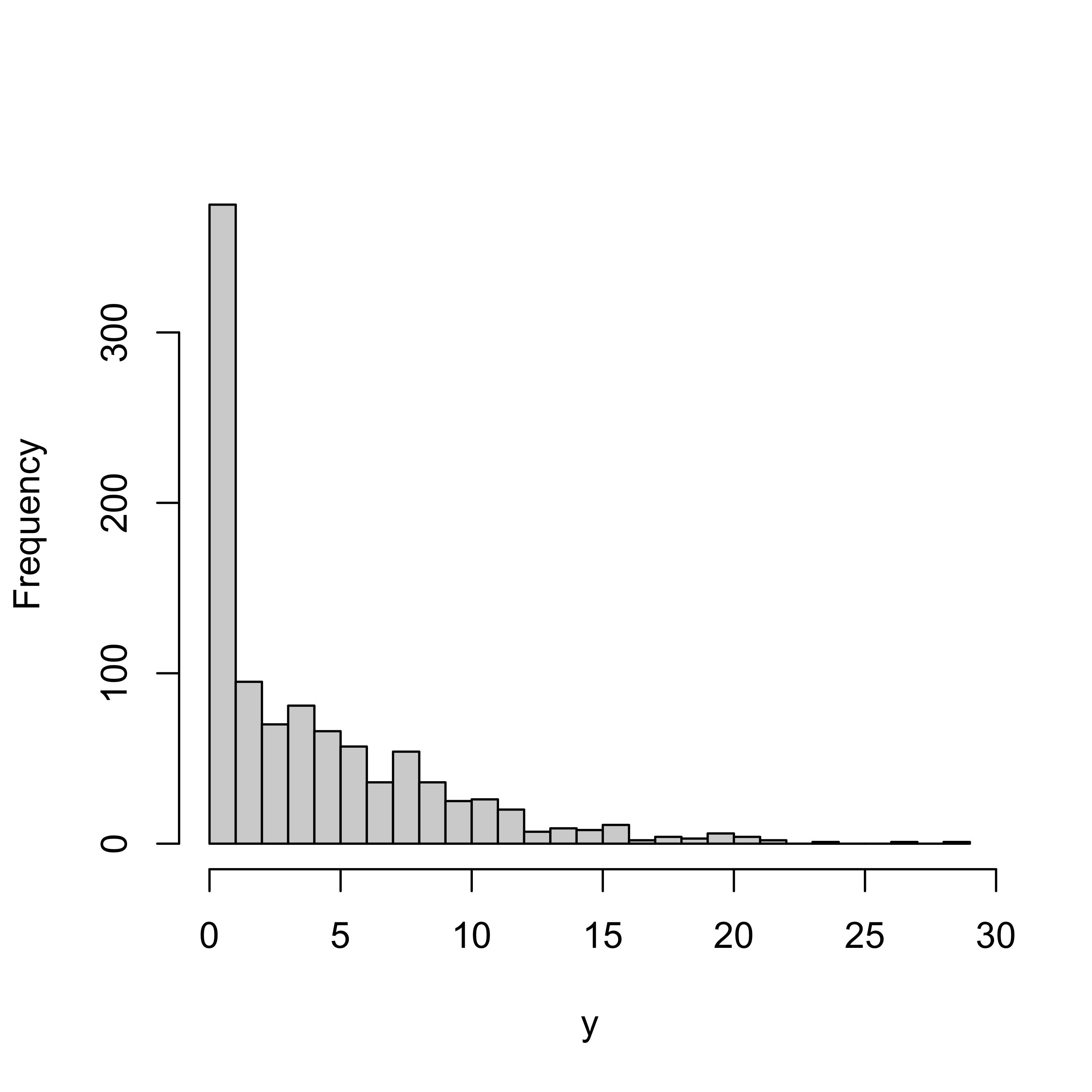
n = 100; phi = 1; mu = 5
theta.t = rgamma(n,phi,phi/mu)
y = rpois(n, theta.t)
a = 1; b = 1;
t.obs = var(y)

nT = 10000
t.pred = rep(NA, nT)
for (t in 1:nT) {
  theta.post = rgamma(1, a + sum(y),
                         b + n)
  y.pred = rpois(n, theta.post)
  t.pred[t] = var(y.pred)
}

hist(t.pred,
     xlim = range(c(t.pred, t.obs)),
     xlab="var",
     main="Posterior Predictive Distribution")

abline(v = t.obs, col="red")Prior/Posterior Checks
STA 702: Lecture 4
Duke University
Uses of Posterior Predictive
Plot the entire density or summarize
Available analytically for conjugate families
Monte Carlo Approximation \[p(y_{n+1} \mid y_1, \ldots y_n) \approx \frac 1 T \sum_{t = 1}^T p(y_{n+1} \mid \theta^{(t)})\] where \(\theta^{(t)} \sim \pi(\theta \mid y_1, \ldots y_n)\) for \(t = 1, \ldots, T\)
T samples from the posterior distribution
Empirical Estimates & Quantiles from Monte Carlo Samples
Models
So far this all assumes we have a correct sampling model and a “reasonable” prior distrbution
George Box: All models are wrong but some are useful
“Useful” \(\rightarrow\) model provides a good approximation; there aren’t clear aspects of the data that are ignored or misspecified
how can we decide if a model is misspecified and needs to change?
Example
Poisson model \[Y_i \mid \theta \stackrel{iid}{\sim }\textsf{Poisson}(\theta) \qquad i = 1, \ldots, n\]
How might our model be misspecified?
Poisson assumes that \(\textsf{E}(Y_i) = \textsf{Var}(Y_i) = \theta\)
it’s very common for data to be over-dispersed \(\textsf{E}(Y_i) < \textsf{Var}(Y_i)\)
ignored additional structure in the data, i.e. data are not iid
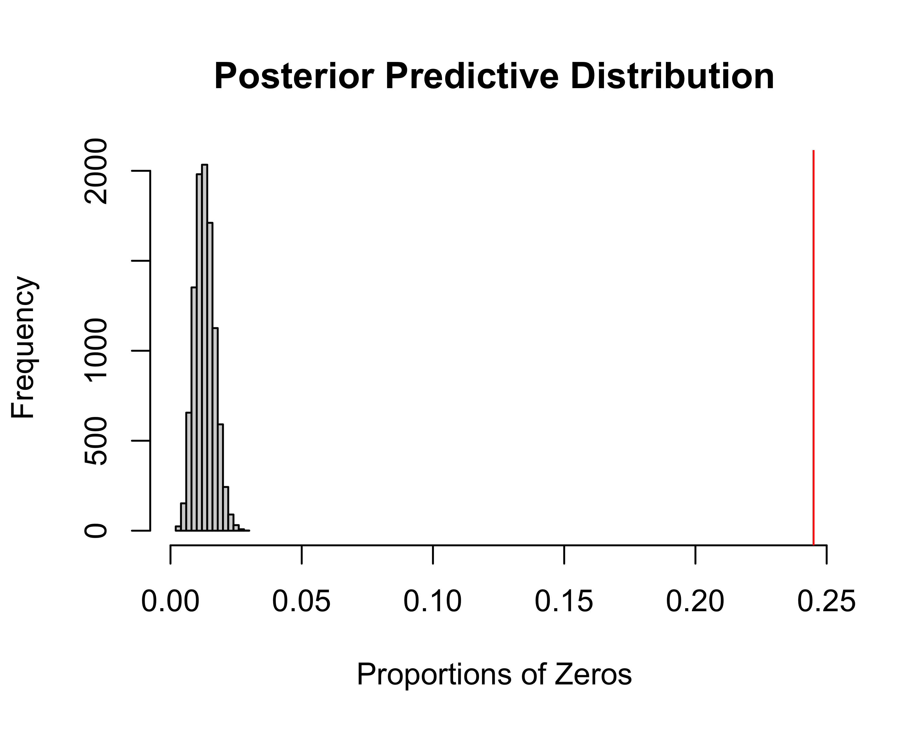
zero-inflation many more zero values than consistent with the poisson model
Posterior Predictive Checks
Guttman (1967), Rubin (1984) proposed the use of Posterior Predictive Checks (PPC)] for model criticism; further developed by Gelman et al (1996)
the spirit of posterior predictive checks is that “If my model is good, then its posterior predictive distribution will generate data that look like my oberved data”
\(y^{\text{obs}}\) is the observed data
\(y^{\text{rep}}\) is a new dataset sampled from the posterior predictive \(p(y^{\text{rep}} \mid y^{\text{obs}})\) of size \(n\) (same size as the observed)
Use a diagnostic statistic \(d(y)\) to capture some feature of the data that the model may fail to capture, say variance
compare \(d(y^{\text{obs}})\) to the reference distribution of \(d(y^{\text{rep}})\)
Use Posterior Predictive P-value as a summary \[ p_{PPC} = P(d(y^{\text{obs}}) > d(y^{\text{rep}}) \mid y^{\text{obs}}) \]
Formally
choose a “diagnostic statistic” \(d(\cdot)\) that captures some summary of the data, e.g. \(\textsf{Var}(y)\) for over-dispersion, where large values of the statistic would be surprising if the model were correct.
\(d(y^{\text{obs}}) \equiv d_{\textrm{obs}}\) value of statistic in observed data
\(d(y^{\text{rep}}_t) \equiv d_{\textrm{pred}}\) value of statistic for the \(t\)th random dataset drawn from the posterior predictive distribution
- Generate \(\theta_t \stackrel{iid}{\sim}p(\theta \mid y^{\textrm{obs}})\)
- Generate \(y^{\textrm{rep}_t} \mid \theta_t \stackrel{iid}{\sim} p(y \mid \theta_t)\)
- Calculate \(d(y^{\text{rep}}_t)\)
plot posterior predictive distribution of \(d(y^{\text{rep}}_t)\) and add \(d_{\textrm{obs}}\)
How extreme is \(t_{\textrm{obs}}\) compared to the distribution of \(d(y^{\text{rep}})\)?
compute p-value \(p_{PPC} = \frac 1 T \sum_t I(d(y^{\text{obs}}) > d(y^{\text{rep}}_t))\)
Example with Over Dispersion
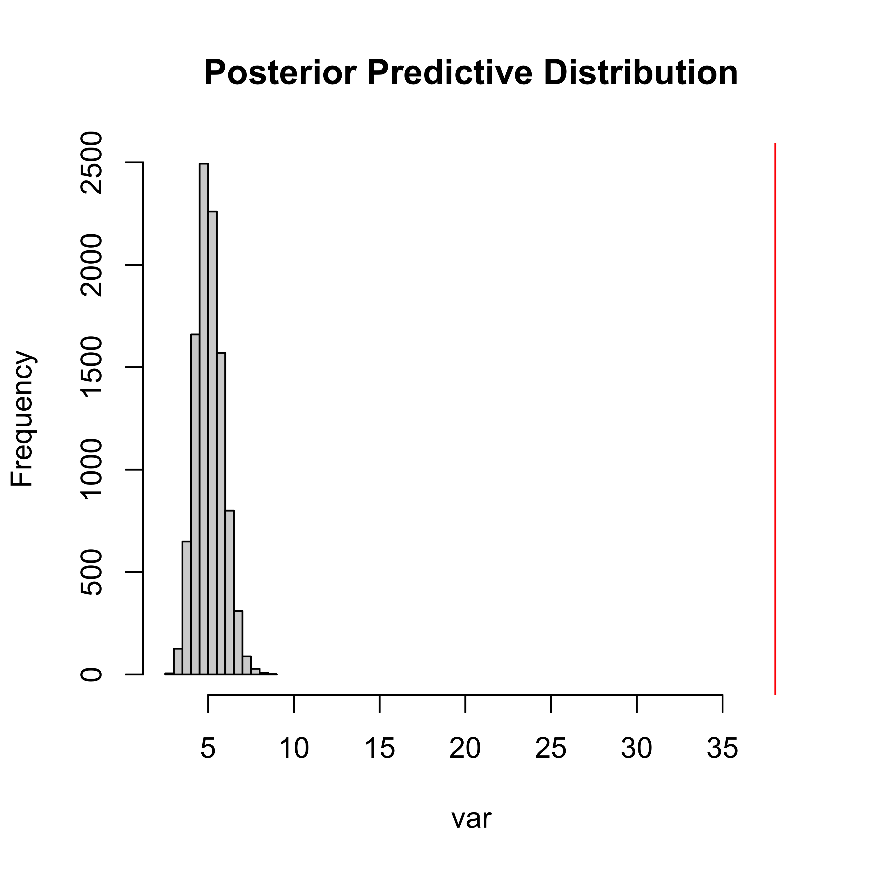
Zero Inflated Distribution
Posterior Predictive Distribution
Posterior Predictive p-values (PPPs)
p-value is probability of seeing something as extreme or more so under a hypothetical “null” model
from a frequentist perspect, one appealing property of p-values is that they should be uniformally distributed under the “null” model
PPPs advocated by Gelman & Rubin in papers and BDA are not valid p-values generally. They are do not have a uniform distribution under the hypothesis that the model is correctly specified
the PPPs tend to be concentrated around 0.5, tend not to reject (conservative)
theoretical reason for the incorrect distribution is due to double use of the data
DO NOT USE as a formal test! use as a diagnostic plot to see how model might fall flat, but be cautious!
Example: Bivariate Normal
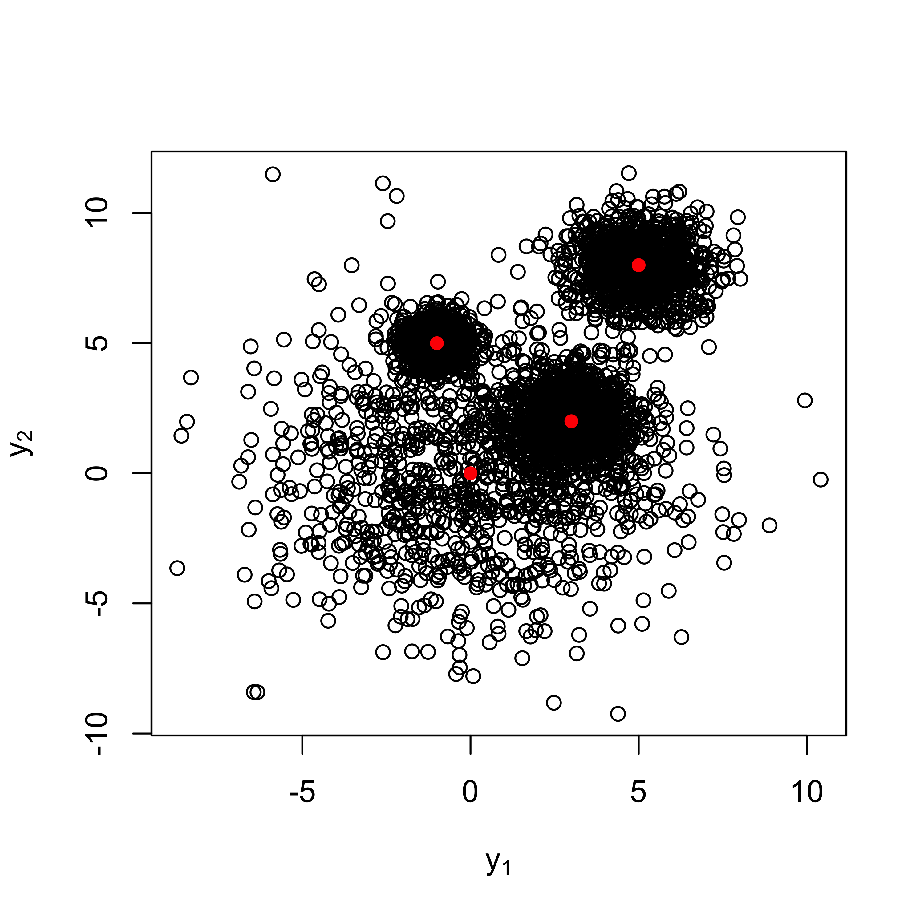
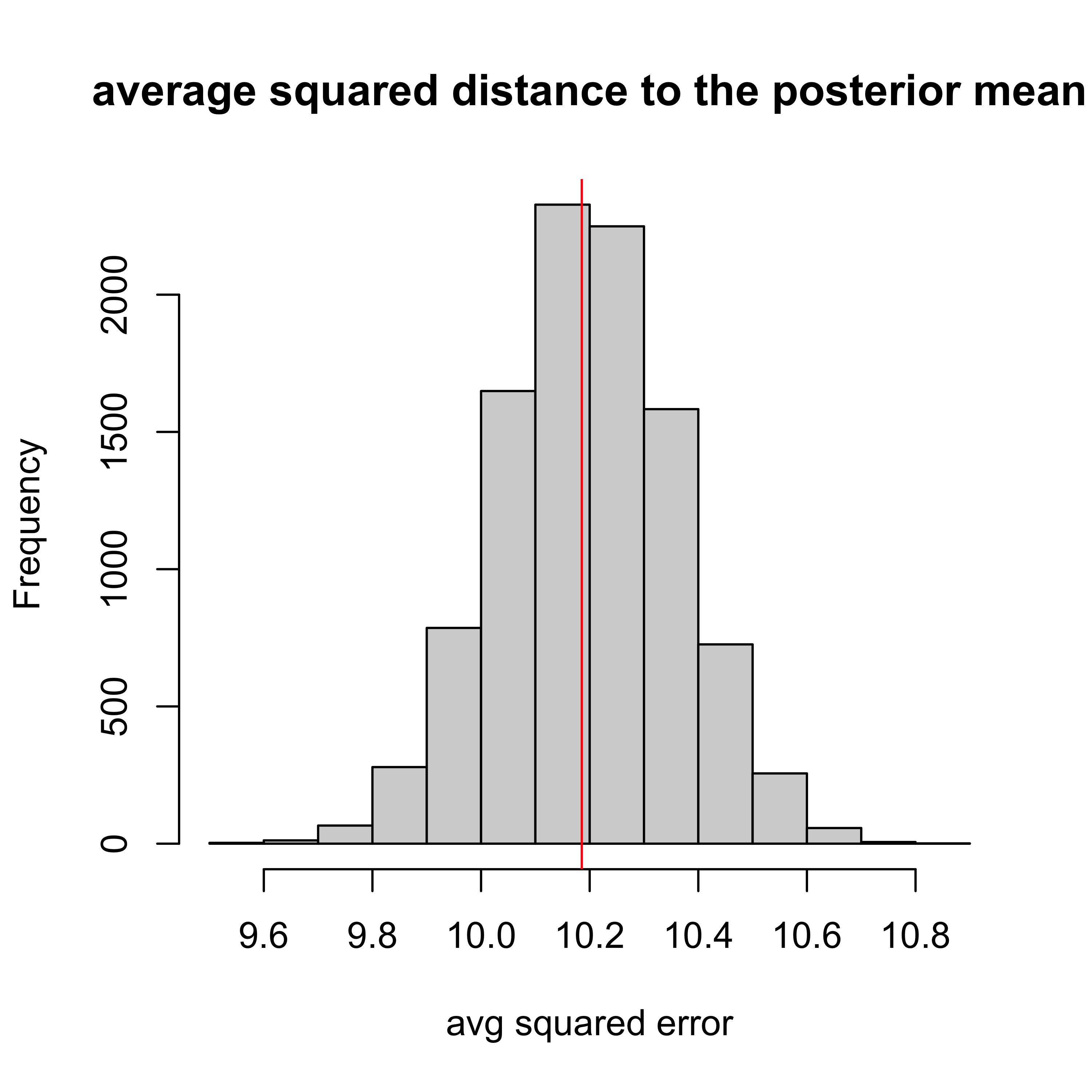
PPP = 0.52
What’s happening?
Problems with PPC
Bayarri & Berger (2000) provides more discussion about why PPP are not always calibrated
Double use of the data; \(Y^{\text{rep}}\) depends on the observed diagnostic in last case
Bayarri & Berger propose partial predictive p-values and conditional predictive p-values that avoid double use of the data by “removing” the contribution of \(d_{\text{obs}}\) to the posterior for \(\theta\) or conditioning on a statistic, such as the MLE of \(\theta\)
heuristically, need the diagnostic to be independent of posterior for \(\theta\) (asymptoptically) under the assumed model
not always easy to find!
Moran et al (2022) propose a workaround to avoid double use of the data by spliting the data \(y_{\text{obs}}, y_{\text{new}}\), use \(y_{\text{obs}}\), to learn \(\theta\) and the other to calculate \(d_{\textrm{new}}\)
can be calculated via simulation easily
POP-PC of Moran et al
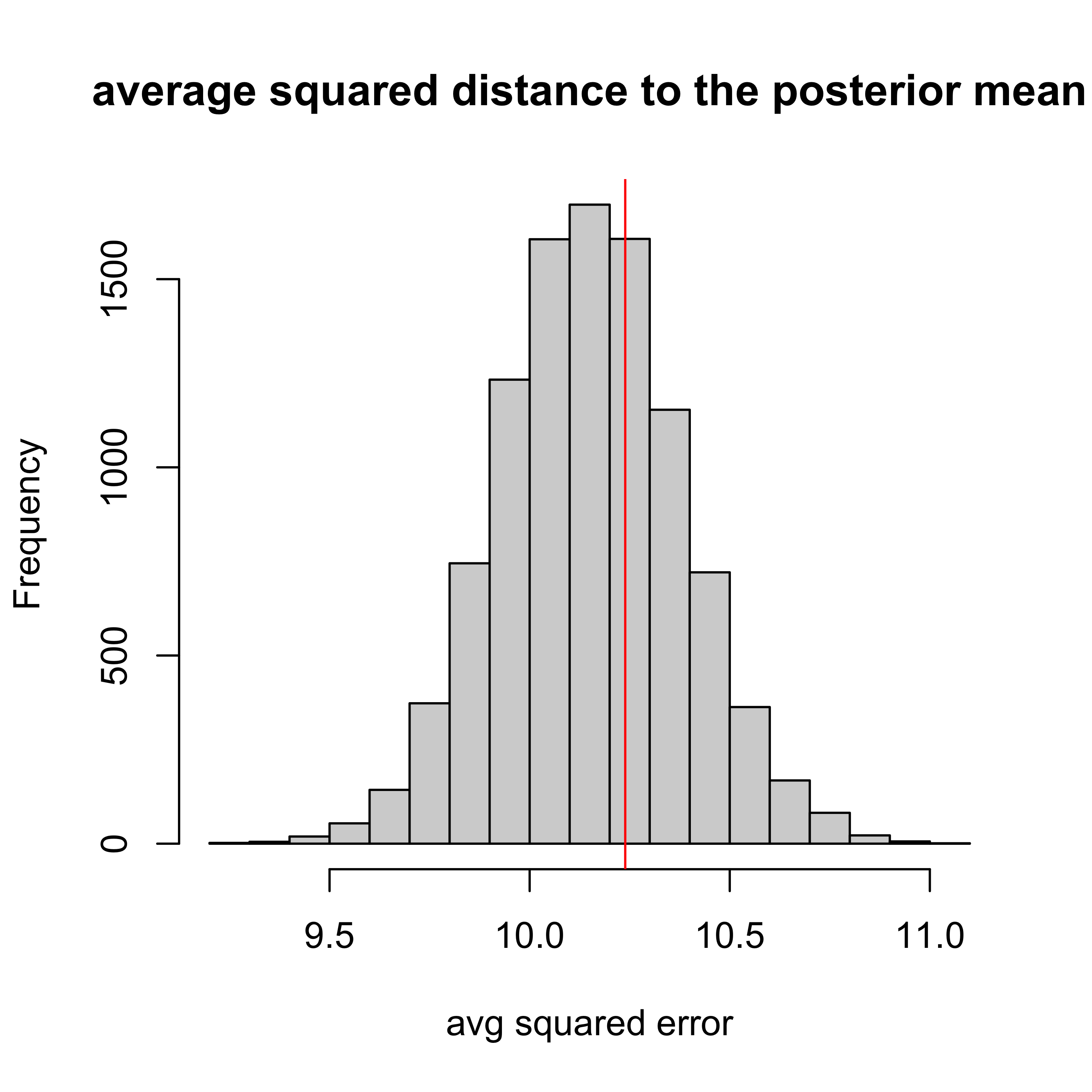
- POP-PPC = 0.35
Modeling Over-Dispersion
Original Model \(Y_i \mid \theta \sim \textsf{Poisson}(\theta)\)
cause of overdispersion is variation in the rate \[ Y_i \mid \theta_i \sim \textsf{Poisson}(\theta_i)\]
model variation via prior \[\theta_i \sim \pi_\theta()\]
\(\pi_\theta()\) characterizes variation in the rate parameter across inviduals
Simple Two Stage Hierarchical Model
Modeling Perspectives
- start with a simple model
- ask if there are surprises through Posterior Checks
- need calibrated diagnostic(s) with good power
- need these to work even if starting model is relatively complex
- other informal diagnostics (residuals)
- remodel if needed based on departures
- Bayesian meaning?
- start with a fairly complex model or models
- shrinkage to prevent overfitting
- formal tests for simplifying models
- methods to combine multiple models to express uncertaity
- properties
Example
\[\theta_i \sim \textsf{Gamma}(\phi \mu, \phi)\]
Find pmf for \(Y_i \mid \mu, \phi\)
Find \(\textsf{E}[Y_i \mid \mu, \phi]\) and \(\textsf{Var}[Y_i \mid \mu, \phi]\)
Homework: \[\theta_i \sim \textsf{Gamma}(\phi, \phi/\mu)\]
Can either of these model zero-inflation?
