Loss Functions, Bayes Risk and Posterior Summaries

STA 702: Lecture 2

Merlise Clyde

Duke University

Last Time …

• Introduction to “ingredients” of Bayesian analysis

• Illustrated a simple Beta-Binomial conjugate example

• Posterior \(\pi(\theta \mid y)\) is a \(\textsf{Beta}(a + y, b + n - y )\)

Today …

• an introduction to loss functions

• Bayes Risk

• optimal decisions and estimators

Bayes estimate

• As we’ve seen by now, having posterior distributions instead of one-number summaries is great for capturing uncertainty.

• That said, it is still very appealing to have simple summaries, especially when dealing with clients or collaborators from other fields, who desire one.

  • What if we want to produce a single “best” estimate of \(\theta\)?

  • What if we want to produce an interval estimate \((\theta_L, \theta_U )\)?

These would provide alternatives to the frequentist MLEs and confidence intervals

Heuristically

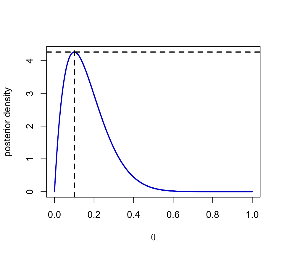
• “best” estimate of \(\theta\) is the maximum a posteriori estimate (MAP) or posterior mode

  • what do we really mean by “best”?

• find an interval such that \(P(\theta \in ( \theta_L, \theta_U ) \mid y) = 1- \alpha\)

  • lots of intervals that satisfy this! which one is “best”?

Loss Functions for Estimators

Introduce loss functions for decision making about what to report!

• a loss function provides a summary for how bad an estimator \(\hat{\theta}\) is relative to the “true” value of \(\theta\)

• Squared error loss \((L2)\)
  \[l(\theta, \hat{\theta}) = (\hat{\theta} - \theta)^2\]

• Absolute error loss \((L1)\) \[l(\theta, \hat{\theta}) = |\hat{\theta} - \theta|\]

But how do we deal with the fact that we do not know \(\theta\)?

Bayes Risk

• Bayes risk is defined as the expected loss of using \(\hat{\theta}\) averaging over the posterior distribution. \[ R(\hat{\theta}) = \textsf{E}_{\pi(\theta \mid y)} [l(\theta, \hat{\theta}) ]\]

• the Bayes optimal estimate \(\hat{\theta}\) is the estimator that has the lowest posterior expected loss or Bayes Risk

• Depends on choice of loss function

• Frequentist risk also exists for evaluating a given estimator under true value of \(\theta\) \[\textsf{E}_{p(y \mid \theta_{\textrm{true}})} [l(\theta_{\textrm{true}} , \hat{\theta}) )]\]

Squared Error Loss

A common choice for point estimation is squared error loss:

\[R(\hat{\theta}) = \textsf{E}_{\pi(\theta \mid y)} [l(\theta, \hat{\theta}) ] = \int_\Theta (\hat{\theta} - \theta)^2 \pi(\theta \mid y) \, d\theta\]

Let’s work it out!

Expand, take expectations of \(R(\hat{\theta})\) with respect to \(\theta\) and factor as a quadratic to find the minimizer (or take derivatives)

Steps

\[R(\hat{\theta}) = \int_\Theta (\hat{\theta}^2 - 2 \hat{\theta} \theta + \theta^2) \pi(\theta \mid y) \, d \theta\]

\[R(\hat{\theta}) = \hat{\theta}^2 - 2 \hat{\theta} \int_\Theta \theta \pi(\theta \mid y) \, d\theta + \int_\Theta \theta^2 \pi(\theta \mid y) \, d\theta\]

\[R(\hat{\theta}) = \hat{\theta}^2 - 2 \hat{\theta} \textsf{E}[\theta \mid y] + \textsf{E}[\theta^2 \mid y]\]

\[R(\hat{\theta}) = \hat{\theta}^2 - 2 \hat{\theta} \textsf{E}[\theta \mid y] + \textsf{E}[\theta \mid y]^2 - \textsf{E}[\theta \mid y]^2 + \textsf{E}[\theta^2 \mid y]\]

Quadratic in \(\hat{\theta}\) minimized when \(\hat{\theta} = \textsf{E}[\theta \mid y]\)
\(\Rightarrow\) posterior mean is the Bayes optimal estimator for \(\theta\) under squared error loss

• In the beta-binomial case for example, the optimal Bayes estimate under squared error loss is \(\hat{\theta} = \frac{a+y}{a+b+n}\)

What about other loss functions?

• Clearly, squared error is only one possible loss function. An alternative is absolute loss, which has \[l(\theta, \hat{\theta}) = |\theta - \hat{\theta}|\]

• Absolute loss places less of a penalty on large deviations & the resulting Bayes estimate is the posterior median.

• Median is actually relatively easy to estimate.

• Recall that for a continuous random variable \(Y\) with cdf \(F\), the median of the distribution is the value \(z\), which satisfies \[F(z) = \Pr(Y\leq z) = \dfrac{1}{2}= \Pr(Y\geq z) = 1-F(z)\]

• As long as we know how to evaluate the CDF of the distribution we have, we can solve for \(z\).

Beta-Binomial

• For the beta-binomial model, the CDF of the beta posterior can be written as \[F(z) = \Pr(\theta\leq z | y) = \int^z_0 \textrm{Beta}(\theta| a+y, b+n-y) d\theta.\]

• Then, if \(\hat{\theta}\) is the median, we have that \(F(\hat{\theta}) = 0.5\)

• To solve for \(\hat{\theta}\), apply the inverse CDF \[\hat{\theta} = F^{-1}(0.5)\]

• In R, that’s simply

qbeta(0.5,a+y,b+n-y)

• For other distributions, switch out the beta.

Loss Functions in General

• A loss function \(l(\theta, \delta(y) )\) is a function of the parameter \(\theta\) and \(\delta(y)\) based on just the data \(y\)

• For example, \(\delta(y) = \bar{y}\) can be the decision to use the sample mean to estimate \(\theta\), the true population mean.

• \(l(\theta, \delta(y) )\) determines the penalty for making the decision \(\delta(y)\), if \(\theta\) is the true parameter or state of nature; the loss function characterizes the price paid for errors.

• Bayes optimal estimator or action is the estimator/action that minimizes the expected posterior loss marginalizing out any unknowns over posterior/predictive distribution.

MAP Estimator

• What about the MAP estimator? Is it an optimal Bayes estimator & under what choice of loss function?

• \(L_\infty\) loss: \[R_{\infty}(\hat{\theta}) = \lim_{p \to \infty} \int_\Theta (\theta - \hat{\theta})^p \pi(\theta \mid y) \, d \theta\]

• Essentially saying that we need the estimator to be right on the truth or the error blows up!

• Is this a reasonable loss function?

Interval Estimates

Recall that a frequentist confidence interval \([l(y), \ u(y)]\) has 95% frequentist coverage for a population parameter \(\theta\) if, before we collect the data, \[\Pr[l(y) < \theta < u(y) | \theta] = 0.95.\]

• This means that 95% of the time, our constructed interval will cover the true parameter, and 5% of the time it won’t.

• There is NOT a 95% chance your interval covers the true parameter once you have collected the data.

• In any given sample, you don’t know whether you’re in the lucky 95% or the unlucky 5%. You just know that either the interval covers the parameter, or it doesn’t (useful, but not too helpful clearly).

• Often based on aysmptotics i.e use a Wald or other type of frequentist asymptotic interval \(\hat{\theta} \pm 1.96 \,\text{se}(\hat{\theta})\)

Bayesian Intervals

• We want a Bayesian alternative to confidence intervals for some pre-specified value of \(\alpha\)

• An interval \([l(y), \ u(y)]\) has \(1 - \alpha\) 100% Bayesian coverage for \(\theta\) if \[\Pr(\theta \in [l(y), \ u(y)] \mid y) = 1 - \alpha\]

• This describes our information about where \(\theta\) lies after we observe the data.

• Fantastic! This is actually the interpretation people want to give to the frequentist confidence interval.

• Bayesian interval estimates are often generally called credible intervals or credible sets.

How to choose \([l(y), \ u(y)]\)?

Bayesian Equal Tail Interval

• The easiest way to obtain a Bayesian interval estimate is to use posterior quantiles with equal tail areas. Often when researchers refer to a credible interval, this is what they mean.

• To make a \(100 \times (1-\alpha)%\) equi-tail quantile-based credible interval, find numbers (quantiles) \(\theta_{\alpha/2} < \theta_{1-\alpha/2}\) such that

  1. \(\Pr(\theta < \theta_{\alpha/2} \mid y) = \dfrac{\alpha}{2}\); and

  2. \(\Pr(\theta > \theta_{1-\alpha/2} \mid y) = \dfrac{\alpha}{2}\).

Convenient conceptually and easy as we just take the \(\alpha/2\) and \(1 - \alpha/2\) quantiles of \(\pi(\theta \mid y)\) as \(l(y)\) and \(u(y)\), respectively.

Beta-Binomial Equal-tailed Interval

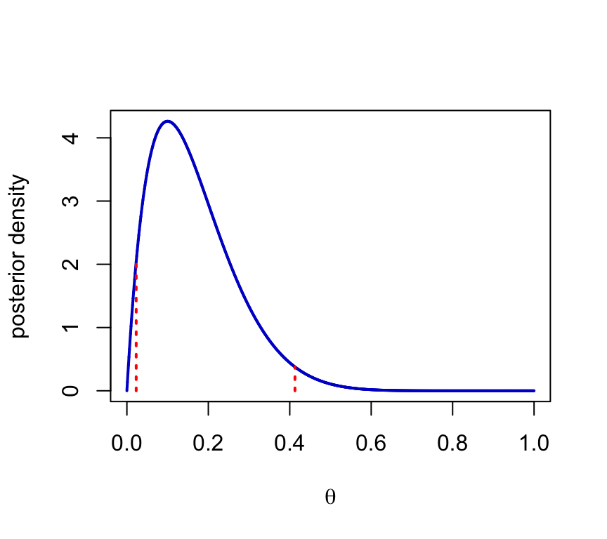
95% Equal -Tail Area interval is \((0.02, 0.41)\)

Monte Carlo Version

• Suppose we don’t have \(\pi(\theta \mid y)\) is a simple form, but we do have samples \(\theta_1, \ldots, \theta_T\) from \(\pi(\theta \mid y)\)

• We can use these samples to obtain Monte Carlo (MC) estimates of posterior summaries \[\hat{\theta} = \textsf{E}[\theta \mid y] \approx \frac{1}{T} \sum_{t= 1}^T \theta_t\]

• what about MC quantile estimates?

• Find the 2.5th and 97.5th percentile from the empirical distribution

theta = rbeta(1000, a + y, b + n - y)
quantile(theta, c(0.025, 0.975))

      2.5%      97.5% 
0.02141993 0.39572970 

Equal-Tail Interval

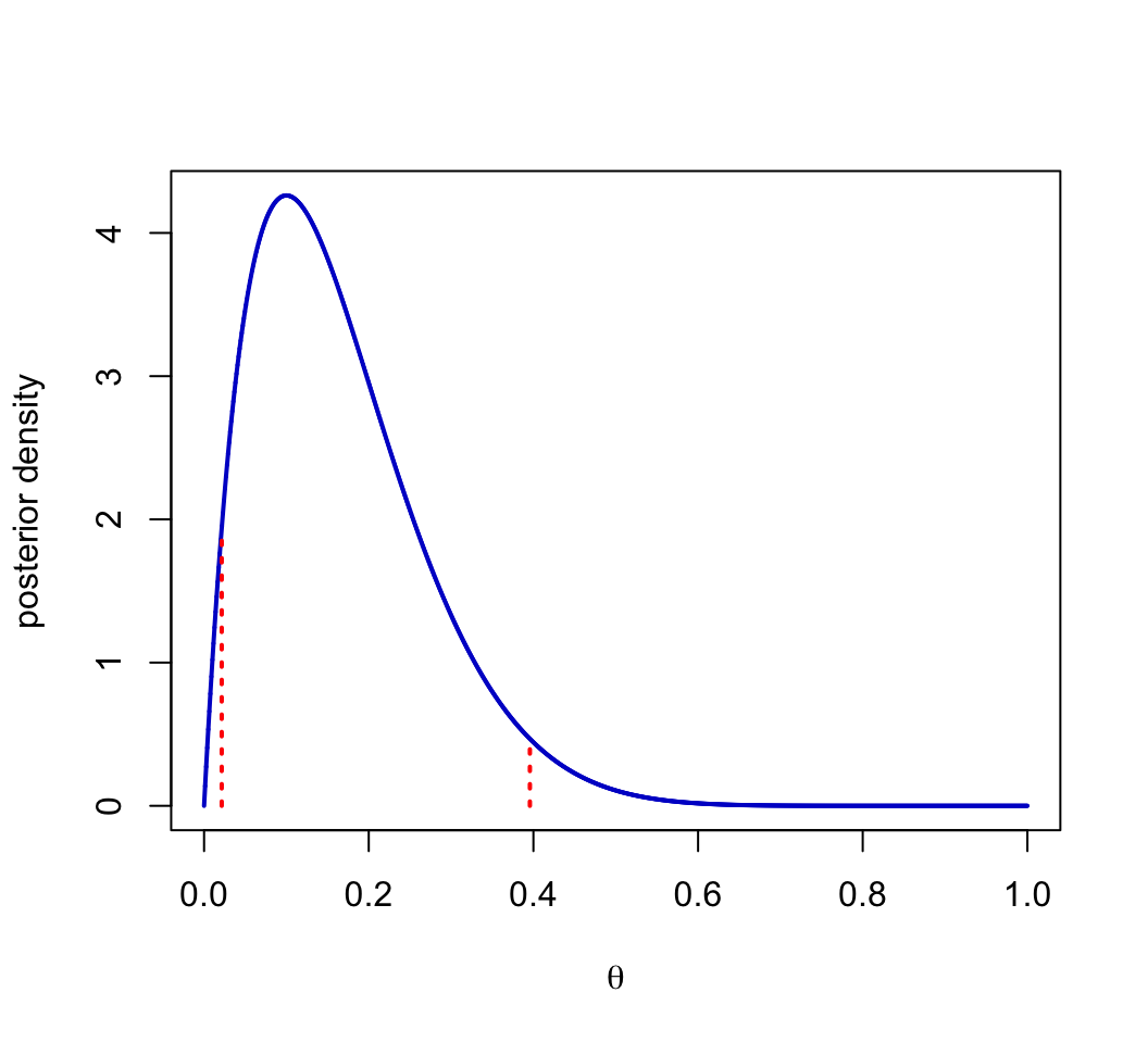
Note there are values of \(\theta\) outside the quantile-based credible interval, with higher density than some values inside the interval.

HPD Region

• A \(100 \times (1-\alpha)%\) highest posterior density (HPD) region is a subset \(s(y)\) of the parameter space \(\Theta\) such that

  1. \(\Pr(\theta \in s(y) \mid y) = 1-\alpha\); and

  2. If \(\theta_a \in s(y)\) and \(\theta_b \notin s(y)\), then \(p(\theta_a \mid y) > p(\theta_b \mid y)\) (highest density set)

• \(\Rightarrow\) All points in a HPD region have higher posterior density than points outside the region.

• The basic idea is to gradually move a horizontal line down across the density, including in the HPD region all values of \(\theta\) with a density above the horizontal line.

• Stop moving the line down when the posterior probability of the values of \(\theta\) in the region reaches \(1-\alpha\).

Simulation Based using the coda Package

 

 

library(coda)
HPDinterval(as.mcmc(theta))

           lower     upper
var1 0.005930904 0.3669906
attr(,"Probability")
[1] 0.95

Properties of HPD Sets

• Shortest length interval (or volume) for the given coverage

• Equivalent to Equal-Tail Intervals if the posterior is unimodal and symmetric

• May not be an interval if the posterior distribution is multi-modal

• In general, not invariant under monotonic transformations of \(\theta\). (Why?)

• More computationally intensive to solve exactly!

See “The Bayesian Choice” by Christian Robert Section 5.5.5 for more info on Loss Functions for Interval Estimation

Connections between Bayes and MLE Based Frequentist Inference

Berstein von Mises (BvM) Theorems) aka Bayesian Central Limit Theorems

• examine limiting form of the posterior distribution \(\pi(\theta \mid y)\) as \(n \to \infty\)

• \(\pi(\theta \mid y)\) goes to a Gaussian under regularity conditions

  • centered at the MLE

  • variance given by the inverse of the Expected Fisher Information (var of MLE)

• The most important implication of the BvM is that Bayesian inference is asymptotically correct from a frequentist point of view

• Used to justify Normal Approximations to the posterior distribution (eg Laplace approximations)

Model Misspecification ?

• We might have chosen a bad sampling model/likelihood

• posterior still converges to a Gaussian centered at the MLE under the misspecified model, but wrong variance

• 95% Bayesian credible sets do not have correct frequentist coverage

• See Klein & van der Vaart for more rigorous treatment if interested

• parametric model is “close” to the true data-generating process

• model diagnostics & changing the model can reduce the gap between model we are using and the true data generating process