Basics of Bayesian Statistics
STA 702: Lecture 1
Duke University
Ingredients
Prior Distribution \(\pi(\theta)\) for unknown \(\theta\)
Likelihood Function \({\cal{L}}(\theta \mid y ) \propto p(y \mid \theta)\) (sampling model)
Posterior Distribution \[\pi(\theta | y) = \frac{\pi(\theta)p(y \mid \theta)}{\int_{\Theta}\pi({\theta})p(y\mid {\theta}) \textrm{d}{\theta}} = \frac{\pi(\theta)p(y\mid\theta)}{p(y)}\]
Loss Function Depends on what you want to report; estimate of \(\theta\), predict future \(Y_{n+1}\), etc
Posterior Depends on Likelihoods
Likelihood function is defined up to a consant \[c \, {\cal{L}}(\theta \mid Y) = p(y \mid \theta) \]
Bayes’ Rule \[\pi(\theta | y) = \frac{\pi(\theta)p(y \mid \theta)}{\int_{\Theta}\pi({\theta})p(y\mid {\theta}) \textrm{d}{\theta}} = \frac{\pi(\theta)c {\cal{L}}(\theta \mid y)}{\int_{\Theta}\pi({\theta})c{\cal{L}}(\theta \mid y) \textrm{d}{\theta}} = \frac{\pi(\theta){\cal{L}}(\theta \mid y)}{m(y)}\]
\(m(y)\) is proportional to the marginal distribution of data
\[m(y) = \int_{\Theta}\pi({\theta}){\cal{L}}(\theta \mid y) \textrm{d}{\theta}\]marginal likelihood of this model or “evidence”
Note: the marginal likelihood and maximized likelihood are very different!
Binomial Example
Binomial sampling \(Y \mid n, \theta \sim \textsf{Binomial}(n, \theta)\)
Probability Mass Function \[p(y \mid \theta) = {n \choose y} \theta^y(1-\theta)^{n-y}\]
Likelihood \(\cal{L}(\theta ) = \theta^y(1-\theta)^{n-y}\)
MLE \(\hat{\theta}\) of Binomial is \(\bar{y} = y/n\) proportion of successes
Recall Derivation!
Marginal Likelihood
\[m(y) = \int_\Theta \cal{L}(\theta) \pi(\theta) \textrm{d}\theta= \int_\Theta \theta^y(1-\theta)^{n-y} \pi(\theta) \textrm{d}\theta\]
“Averaging” of likelihood over prior \(\pi(\theta) = 1\)

Binomial Example
Prior \(\theta \sim \textsf{U}(0,1)\) or \(\pi(\theta) = 1, \quad \textrm{for } \theta \in (0,1)\)
Marginal \(m(y) = \int_0^1 \theta^y(1-\theta)^{n-y}\, 1 \,\textrm{d}\theta\)
Special function known as the beta function - see Rudin \[{B}(a, b) = \int_0^1 \theta^{a - 1}(1-\theta)^{b - 1} \,\textrm{d}\theta \]
Posterior Distribution \[\pi(\theta \mid y ) = \frac{ \theta^{(y+1)-1} (1-\theta)^{(n - y +1) -1}}{B(y + 1,n - y + 1)}\]
\[\theta \mid y \sim \textsf{Beta}(y + 1, n - y + 1) \]
Beta Prior Distributions
\(\textsf{Beta}(a, b)\) is a probability density function (pdf) on (0,1),
\[\pi(\theta) = \frac{1}{B(a,b)} \theta^{a-1} (1-\theta)^{b -1}\]
Use the kernel trick to find the posterior \[\pi(\theta \mid y) \propto \cal{L}(\theta \mid y) \pi(\theta)\]
Write down likelihood and prior (ignore constants wrt \(\theta\))
Recognize kernel of density
Figure out normalizing constant/distribution
Try it!
Prior to Posterior Updating Binomial Data
Prior \(\textsf{Beta}(a, b)\)
Posterior \(\textsf{Beta}(a + y, b + n - y)\)
Conjugate prior & posterior distribution are in the same family of distributions, (Beta)
Simple updating of information from the prior to posterior
\(a + b\) “prior sample size” (number of trials in a hypothetical experiment)
\(a\) “number of successes”
\(b\) “number of failures”
prior elicitation (process of choosing the prior hyperparamters) based on historic or imaginary data
Summaries & Properties
For \(\theta \sim \textsf{Beta}(a,b)\) let \(a + b = n_0\) “prior sample size”
Prior mean \[\textsf{E}[\theta] = \frac{a}{a+b} \equiv \theta_0 \]
Posterior mean \[\textsf{E}[\theta \mid y ] = \frac{a + y }{a+b +n} \equiv \tilde{\theta} \]
Rewrite with MLE \(\hat{\theta} = \bar{y} = \frac{y}{n}\) and prior mean \[\textsf{E}[\theta \mid y ] = \frac{a + y }{a+b +n} = \frac{n_0}{n_0 + n} \theta_0 + \frac{n}{n_0 + n} \hat{\theta}\]
Weighted average of prior mean and MLE where weight for \(\theta_0 \propto n_0\) and weight for \(\hat{\theta} \propto n\)
Properties
Posterior mean \[\tilde{\theta} = \frac{n_0}{n_0 + n} \theta_0 + \frac{n}{n_0 + n} \hat{\theta}\]
in finite samples we get shrinkage: posterior mean pulls the MLE toward the prior mean; amount depends on prior sample size \(n_0\) and data sample size \(n\)
regularization effect to reduce Mean Squared Error for estimation with small sample sizes and noisy data
introduces some bias (in the frequentist sense) due to prior mean \(\theta_0\)
reduces variance (bias-variance trade-off)
helpful in the Binomial case, when sample size is small or \(\theta_{\text{true}} \approx 0\) (rare events) and \(\hat{\theta} = 0\) (inbalanced categorical data)
as we get more information from the data \(n \to \infty\) we have \(\tilde{\theta} \to \hat{\theta}\) and consistency ! As \(n \to \infty, \textsf{E}[\tilde{\theta}] \to \theta_{\text{true}}\)
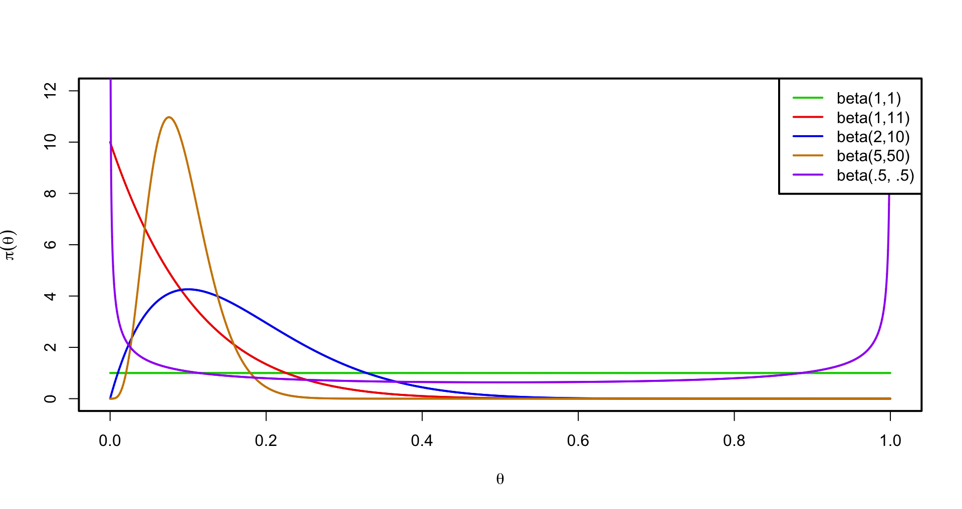
Some possible prior densities

Prior Choice
Is the uniform prior \(\textsf{Beta}(1,1)\) non-informative?
- No- if \(y = 0\) (or \(n\)) sparse/rare events saying that we have a prior “historical” sample with 1 success and 1 failure ( \(a = 1\) and \(b = 1\) ) can be very informative
What about a uniform prior on the log odds? \(\eta \equiv \log\left( \frac{\theta} {1 - \theta} \right)\)? \[\pi(\eta) \propto 1, \qquad \eta \in \mathbb{R}\]
Is this a proper prior distribution?
what would be induced measure for \(\theta\)?
Find Jacobian (exercise!) \[\pi(\theta) \propto \theta^{-1} (1 - \theta)^{-1}, \qquad \theta \in (0,1)\]
limiting case of a Beta \(a \to 0\) and \(b \to 0\) (Haldane’s prior)
Formal Bayes
use of improper prior and turn the Bayesian crank
calculate \(m(y)\) and renormalize likelihood times “improper prior” if \(m(y)\) is finite
formal posterior is \(\textsf{Beta}(y, n-y)\) and reasonable only if \(y \neq 0\) or \(y \neq n\) as \(B(0, -)\) and \(B(-, 0)\) (normalizing constant) are undefined!
no shrinkage \(\textsf{E}[\theta \mid y] = \frac{y}{n} = \tilde{\theta} = \hat{\theta}\)
Invariance
Jeffreys argues that priors should be invariant to transformations to be non-informative. . . . i.e. if we reparameterize with \(\theta = h(\rho)\) then the rule should be that \[\pi_\theta(\theta) = \left|\frac{ d \rho} {d \theta}\right| \pi_\rho(h^{-1}(\theta))\]
Jefferys’ rule is to pick \(\pi(\rho) \propto (I(\rho))^{1/2}\)
Expected Fisher Information for \(\rho\) \[ I(\rho) = - \textsf{E} \left[ \frac {d^2 \log ({\cal{L}}(\rho))} {d^2 \rho} \right]\]
For the Binomial example \(\pi(\theta) \propto \theta^{-1/2} (1 - \theta)^{-1/2}\)
Thus Jefferys’ prior is a \(\textsf{Beta}(1/2, 1/2)\)
Why ?
Chain Rule!
Find Jefferys’ prior for \(\theta\) where \(Y \sim \textsf{Ber}(\theta)\)
Find information matrix \(I(\rho)\) for \(\rho = \rho(\theta)\) from \(I(\theta)\)
Show that the prior satisfies the invariance property!
Find Jeffreys’ prior for \(\rho = \log(\frac{\theta}{1 - \theta})\)